Summarise cohort timing • CohortCharacteristics

We saw in the previous vignette how we can summarise the overlap between cohorts. In addition to this, we might also be interested in timings between cohorts. That is, the time between an individual entering one cohort and another. For this we can use the summariseCohortTiming(). In this example we’ll look at the time between entering cohorts for acetaminophen, morphine, and oxycodone using the Eunomia data.

library(duckdb)
library(CDMConnector)
library(dplyr, warn.conflicts = FALSE)
library(CodelistGenerator)
library(PatientProfiles)
library(CohortCharacteristics)

con <- dbConnect(duckdb(), dbdir = eunomiaDir())
cdm <- cdmFromCon(
  con = con, cdmSchem = "main", writeSchema = "main", cdmName = "Eunomia"
)

medsCs <- getDrugIngredientCodes(
  cdm = cdm,
  name = c(
    "acetaminophen",
    "morphine",
    "warfarin"
  )
)

cdm <- generateConceptCohortSet(
  cdm = cdm,
  name = "meds",
  conceptSet = medsCs,
  end = "event_end_date",
  limit = "all",
  overwrite = TRUE
)

settings(cdm$meds)
#> # A tibble: 3 × 6
#>   cohort_definition_id cohort_name    limit prior_observation future_observation
#>                  <int> <chr>          <chr>             <dbl>              <dbl>
#> 1                    1 11289_warfarin all                   0                  0
#> 2                    2 161_acetamino… all                   0                  0
#> 3                    3 7052_morphine  all                   0                  0
#> # ℹ 1 more variable: end <chr>
cohortCount(cdm$meds)
#> # A tibble: 3 × 3
#>   cohort_definition_id number_records number_subjects
#>                  <int>          <int>           <int>
#> 1                    1            137             137
#> 2                    2          13908            2679
#> 3                    3             35              35

Now we have our cohorts we can summarise the timing between cohort entry. Note setting restrictToFirstEntry to TRUE will mean that we only consider timing between an individual’s first record in each cohort (i.e. their first exposure to each of the medications).

medsTiming <- cdm$meds |>
  summariseCohortTiming(restrictToFirstEntry = TRUE)
medsTiming |>
  glimpse()
#> Rows: 6,186
#> Columns: 13
#> $ result_id        <int> 1, 1, 1, 1, 1, 1, 1, 1, 1, 1, 1, 1, 1, 1, 1, 1, 1, 1,…
#> $ cdm_name         <chr> "Eunomia", "Eunomia", "Eunomia", "Eunomia", "Eunomia"…
#> $ group_name       <chr> "cohort_name_reference &&& cohort_name_comparator", "…
#> $ group_level      <chr> "11289_warfarin &&& 161_acetaminophen", "11289_warfar…
#> $ strata_name      <chr> "overall", "overall", "overall", "overall", "overall"…
#> $ strata_level     <chr> "overall", "overall", "overall", "overall", "overall"…
#> $ variable_name    <chr> "number records", "number subjects", "days_between_co…
#> $ variable_level   <chr> NA, NA, NA, NA, NA, NA, NA, "density_001", "density_0…
#> $ estimate_name    <chr> "count", "count", "min", "q25", "median", "q75", "max…
#> $ estimate_type    <chr> "integer", "integer", "integer", "integer", "integer"…
#> $ estimate_value   <chr> "136", "136", "-33784", "-24462", "-19709", "-16926",…
#> $ additional_name  <chr> "overall", "overall", "overall", "overall", "overall"…
#> $ additional_level <chr> "overall", "overall", "overall", "overall", "overall"…

As with cohort overlap, we have table and plotting functions to help view our results.

tableCohortTiming(medsTiming, timeScale = "years", uniqueCombinations = FALSE)

CDM name	Cohort name reference	Cohort name comparator	Variable name	Estimate name	Estimate value
Eunomia	11289_warfarin	161_acetaminophen	number records	N	136
			number subjects	N	136
			years_between_cohort_entries	Median [Q25 - Q75]	-53.96 [-66.97 - -46.34]
				Range	-92.50 to 3.03
		7052_morphine	number records	N	6
			number subjects	N	6
			years_between_cohort_entries	Median [Q25 - Q75]	-4.54 [-10.36 - 4.76]
				Range	-18.99 to 9.24
	161_acetaminophen	11289_warfarin	number records	N	136
			number subjects	N	136
			years_between_cohort_entries	Median [Q25 - Q75]	53.96 [46.34 - 66.97]
				Range	-3.03 to 92.50
		7052_morphine	number records	N	35
			number subjects	N	35
			years_between_cohort_entries	Median [Q25 - Q75]	15.79 [5.02 - 33.51]
				Range	-33.72 to 77.29
	7052_morphine	11289_warfarin	number records	N	6
			number subjects	N	6
			years_between_cohort_entries	Median [Q25 - Q75]	4.54 [-4.76 - 10.36]
				Range	-9.24 to 18.99
		161_acetaminophen	number records	N	35
			number subjects	N	35
			years_between_cohort_entries	Median [Q25 - Q75]	-15.79 [-33.51 - -5.02]
				Range	-77.29 to 33.72

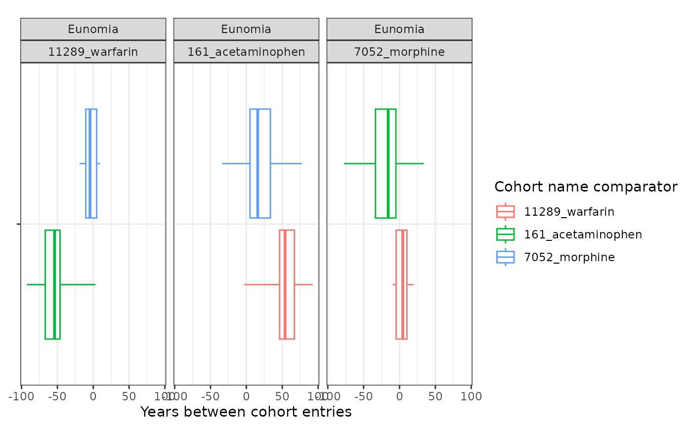
plotCohortTiming(
  medsTiming,
  plotType = "boxplot",
  timeScale = "years",
  uniqueCombinations = FALSE
)

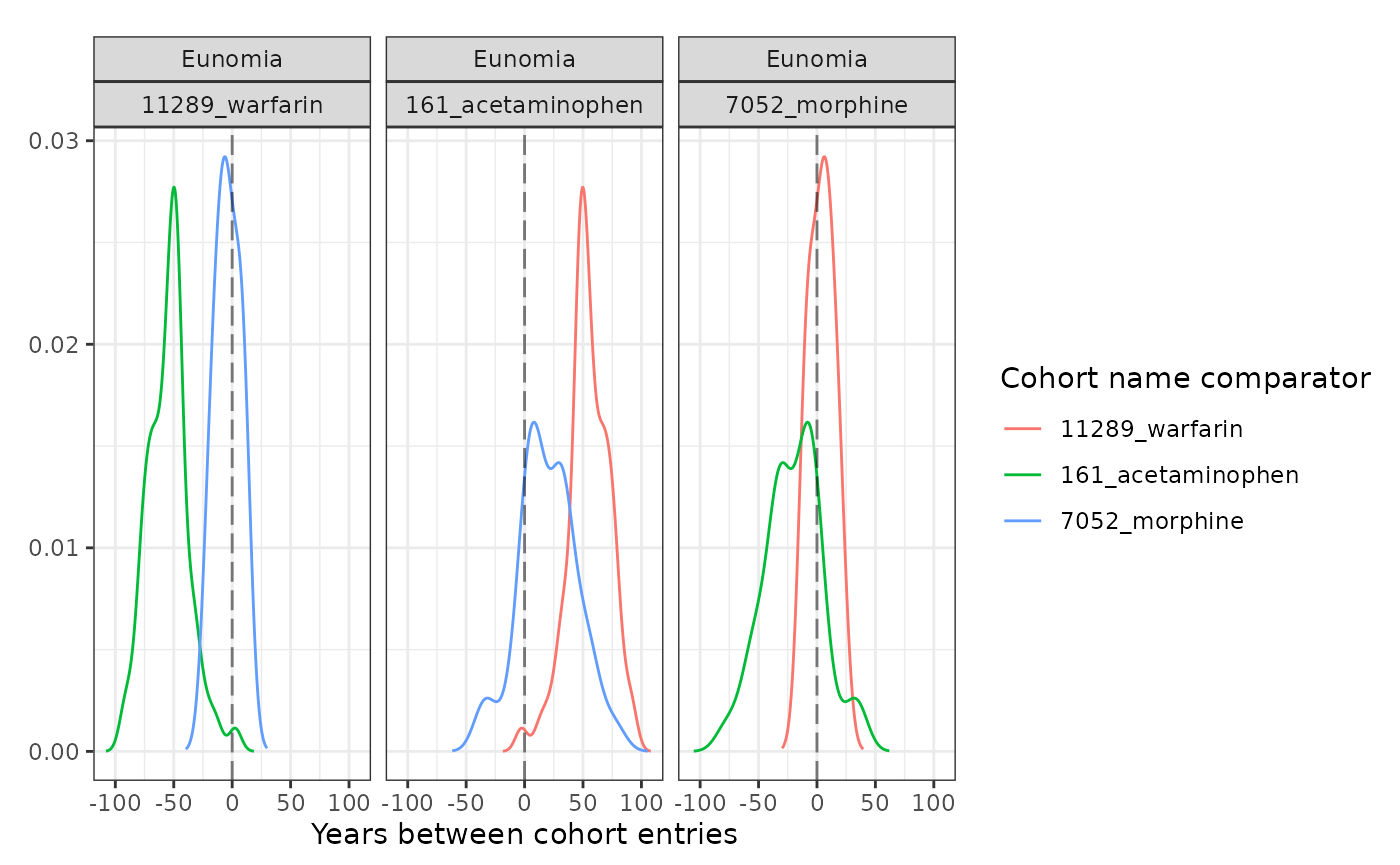
If we want to see an even more granular summary of cohort timings we can make a density plot instead of a box plot. Note, for this we’ll need to set density to include ‘density’ as one of the estimates.

plotCohortTiming(
  medsTiming,
  plotType = "density",
  timeScale = "years",
  uniqueCombinations = FALSE
)

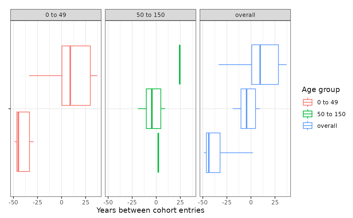
As well as generating these estimates for cohorts overall, we can also obtain stratified estimates.

cdm$meds <- cdm$meds |>
  addAge(ageGroup = list(c(0, 49), c(50, 150))) |>
  compute(temporary = FALSE, name = "meds") |>
  newCohortTable()
medsTiming <- cdm$meds |>
  summariseCohortTiming(
    restrictToFirstEntry = TRUE,
    strata = list("age_group"),
    density = TRUE
  )
tableCohortTiming(medsTiming, timeScale = "years")

CDM name	Cohort name reference	Cohort name comparator	Variable name	Estimate name	Age group
CDM name	Cohort name reference	Cohort name comparator	Variable name	Estimate name	overall	0 to 49	50 to 150
Eunomia	11289_warfarin	161_acetaminophen	number records	N	9	8	1
			number subjects	N	9	8	1
			years_between_cohort_entries	Median [Q25 - Q75]	-43.77 [-46.35 - -32.09]	-44.88 [-46.44 - -33.29]	2.12 [2.12 - 2.12]
				Range	-48.89 to 2.12	-48.89 to -29.03	2.12 to 2.12
		7052_morphine	number records	N	6	-	6
			number subjects	N	6	-	6
			years_between_cohort_entries	Median [Q25 - Q75]	-4.54 [-10.36 - 4.76]	-	-4.54 [-10.36 - 4.76]
				Range	-18.99 to 9.24	-	-18.99 to 9.24
	161_acetaminophen	7052_morphine	number records	N	26	25	1
			number subjects	N	26	25	1
			years_between_cohort_entries	Median [Q25 - Q75]	9.55 [0.85 - 28.56]	9.05 [0.41 - 29.90]	24.44 [24.44 - 24.44]
				Range	-33.72 to 37.08	-33.72 to 37.08	24.44 to 24.44

plotCohortTiming(medsTiming,
  plotType = "boxplot",
  timeScale = "years",
  facet = "age_group",
  colour = "age_group",
  uniqueCombinations = TRUE
)