Summarise patient characteristics
Source:vignettes/summarise_characteristics.Rmd
summarise_characteristics.RmdIntroduction
In this example we’re going to summarise the characteristics of individuals with an ankle sprain, ankle fracture, forearm fracture, or a hip fracture using the Eunomia synthetic database.
We’ll begin by creating our condition study cohorts with the
generateConceptCohortSet function from
CDMConnector.
library(omock)
library(CDMConnector)
library(dplyr, warn.conflicts = FALSE)
library(ggplot2)
library(CodelistGenerator)
library(PatientProfiles)
library(CohortCharacteristics)

cdm <- mockCdmFromDataset(datasetName = "GiBleed", source = "duckdb")

cdm <- generateConceptCohortSet(
  cdm = cdm,
  name = "injuries",
  conceptSet = list(
    "ankle_sprain" = 81151,
    "ankle_fracture" = 4059173,
    "forearm_fracture" = 4278672,
    "hip_fracture" = 4230399
  ),
  end = "event_end_date",
  limit = "all"
)
settings(cdm$injuries)
#> # A tibble: 4 × 6
#>   cohort_definition_id cohort_name    limit prior_observation future_observation
#>                  <int> <chr>          <chr>             <dbl>              <dbl>
#> 1                    1 ankle_sprain   all                   0                  0
#> 2                    2 ankle_fracture all                   0                  0
#> 3                    3 forearm_fract… all                   0                  0
#> 4                    4 hip_fracture   all                   0                  0
#> # ℹ 1 more variable: end <chr>
cohortCount(cdm$injuries)
#> # A tibble: 4 × 3
#>   cohort_definition_id number_records number_subjects
#>                  <int>          <int>           <int>
#> 1                    1           1915            1357
#> 2                    2            464             427
#> 3                    3            569             510
#> 4                    4            138             132
Summarising study cohorts
Now we’ve created our cohorts, we can obtain a summary of the characteristics in the patients included in these cohorts. We’ll create two different age group in below example: under 50 and 50+.
chars <- cdm$injuries |>
  summariseCharacteristics(ageGroup = list(c(0, 49), c(50, Inf)))
chars |>
  glimpse()
#> Rows: 220
#> Columns: 13
#> $ result_id        <int> 1, 1, 1, 1, 1, 1, 1, 1, 1, 1, 1, 1, 1, 1, 1, 1, 1, 1,…
#> $ cdm_name         <chr> "GiBleed", "GiBleed", "GiBleed", "GiBleed", "GiBleed"…
#> $ group_name       <chr> "cohort_name", "cohort_name", "cohort_name", "cohort_…
#> $ group_level      <chr> "ankle_sprain", "ankle_sprain", "ankle_sprain", "ankl…
#> $ strata_name      <chr> "overall", "overall", "overall", "overall", "overall"…
#> $ strata_level     <chr> "overall", "overall", "overall", "overall", "overall"…
#> $ variable_name    <chr> "Number records", "Number subjects", "Cohort start da…
#> $ variable_level   <chr> NA, NA, NA, NA, NA, NA, NA, NA, NA, NA, NA, NA, NA, N…
#> $ estimate_name    <chr> "count", "count", "min", "q25", "median", "q75", "max…
#> $ estimate_type    <chr> "integer", "integer", "date", "date", "date", "date",…
#> $ estimate_value   <chr> "1915", "1357", "1912-02-25", "1968-06-15", "1982-11-…
#> $ additional_name  <chr> "overall", "overall", "overall", "overall", "overall"…
#> $ additional_level <chr> "overall", "overall", "overall", "overall", "overall"…
Now we have generated the results, we can create a nice table in gt
format to display the results using tableCharacteristics
function. By default it returns summary statistics for, number records,
number subjects, age, cohort_start_date, cohort_end_date,
prior_observations, future_observations and days in cohort. Days in
cohort is defined as the number of days between the cohort start and end
dates, inclusive of both boundaries (i.e., cohort_end_date –
cohort_start_date + 1). This represents the total duration an individual
in the cohort. In contrast, future observation time is defined as the
time from the cohort start date to the end of the individual’s
observation period (observation_period_end_date – cohort_start_date).
Prior observation works similar to future observation but look at
observations before cohort_start_date, hence defined as
(cohort_start_date - observation_period_start_date). The difference in
definitions arises because days in cohort captures a duration within the
cohort, while future observation time measures a remaining time window
for potential follow-up beyond cohort entry.
tableCharacteristics(chars)|
CDM name
|
||||||
|---|---|---|---|---|---|---|
|
GiBleed
|
||||||
| Variable name | Variable level | Estimate name |
Cohort name
|
|||
| ankle_sprain | ankle_fracture | forearm_fracture | hip_fracture | |||
| Number records | – | N | 1,915 | 464 | 569 | 138 |
| Number subjects | – | N | 1,357 | 427 | 510 | 132 |
| Cohort start date | – | Median [Q25 - Q75] | 1982-11-09 [1968-06-15 - 1999-04-13] | 1981-01-15 [1965-03-11 - 1997-08-03] | 1981-07-24 [1967-03-05 - 2000-12-16] | 1996-09-17 [1977-09-20 - 2010-06-22] |
| Range | 1912-02-25 to 2019-05-30 | 1911-09-07 to 2019-06-23 | 1917-08-16 to 2019-06-26 | 1927-12-14 to 2019-05-08 | ||
| Cohort end date | – | Median [Q25 - Q75] | 1982-12-10 [1968-07-06 - 1999-05-09] | 1981-02-28 [1965-04-11 - 1997-10-12] | 1981-08-23 [1967-04-10 - 2001-02-27] | 1996-11-16 [1977-12-04 - 2010-07-22] |
| Range | 1912-03-10 to 2019-05-30 | 1911-12-06 to 2019-06-24 | 1917-11-14 to 2019-06-26 | 1928-03-13 to 2019-06-07 | ||
| Age | – | Median [Q25 - Q75] | 21 [9 - 41] | 16 [9 - 43] | 17 [9 - 46] | 40 [13 - 66] |
| Mean (SD) | 26.63 (21.03) | 27.38 (24.70) | 28.69 (25.97) | 40.06 (28.82) | ||
| Range | 0 to 105 | 0 to 107 | 0 to 106 | 1 to 108 | ||
| Age group | 0 to 49 | N (%) | 1,587 (82.87%) | 367 (79.09%) | 440 (77.33%) | 87 (63.04%) |
| 50 or above | N (%) | 328 (17.13%) | 97 (20.91%) | 129 (22.67%) | 51 (36.96%) | |
| Sex | Female | N (%) | 954 (49.82%) | 238 (51.29%) | 286 (50.26%) | 74 (53.62%) |
| Male | N (%) | 961 (50.18%) | 226 (48.71%) | 283 (49.74%) | 64 (46.38%) | |
| Prior observation | – | Median [Q25 - Q75] | 7,833 [3,628 - 15,147] | 6,030 [3,360 - 16,032] | 6,289 [3,390 - 16,847] | 14,522 [4,801 - 24,401] |
| Mean (SD) | 9,918.17 (7,672.74) | 10,196.57 (9,011.31) | 10,670.43 (9,480.30) | 14,821.73 (10,521.89) | ||
| Range | 299 to 38,429 | 299 to 39,430 | 299 to 38,943 | 390 to 39,792 | ||
| Future observation | – | Median [Q25 - Q75] | 12,868 [6,860 - 18,078] | 13,748 [6,878 - 19,331] | 13,165 [5,988 - 18,548] | 7,798 [2,874 - 14,913] |
| Mean (SD) | 12,865.11 (7,543.50) | 13,470.92 (8,215.96) | 12,913.27 (7,929.17) | 9,167.33 (7,160.81) | ||
| Range | 0 to 38,403 | 1 to 39,051 | 0 to 36,654 | 0 to 29,045 | ||
| Days in cohort | – | Median [Q25 - Q75] | 22 [15 - 29] | 61 [31 - 91] | 61 [31 - 91] | 61 [31 - 91] |
| Mean (SD) | 25.02 (8.00) | 61.65 (25.38) | 62.16 (25.32) | 59.26 (24.79) | ||
| Range | 1 to 37 | 2 to 92 | 1 to 91 | 1 to 91 | ||
| Days to next record | – | Median [Q25 - Q75] | 6,082 [2,640 - 10,540] | 5,100 [2,430 - 11,474] | 5,760 [1,922 - 15,606] | 7,430 [2,355 - 15,966] |
| Mean (SD) | 7,457.56 (5,937.15) | 7,784.46 (7,686.21) | 9,217.83 (8,826.17) | 9,037.50 (8,138.51) | ||
| Range | 300 to 29,145 | 330 to 28,365 | 360 to 34,482 | 690 to 19,200 | ||
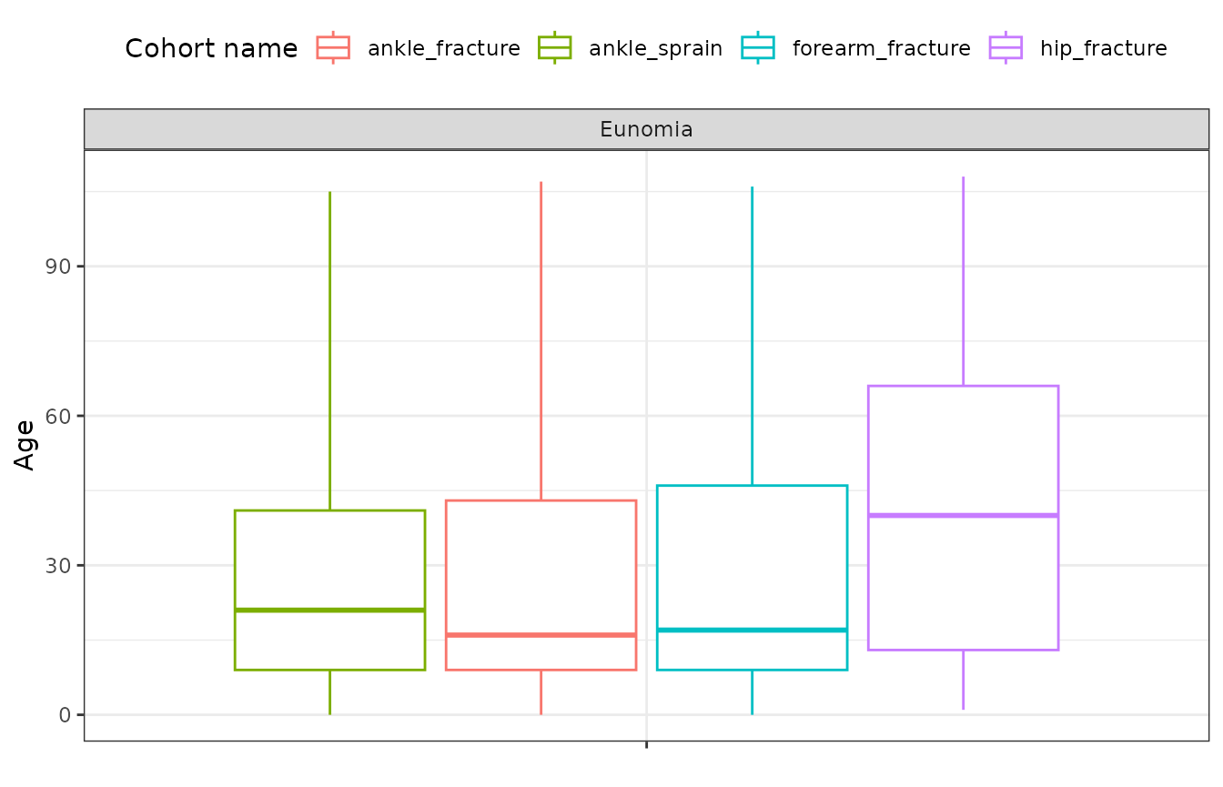
We can also use the plotCharacteristics function to
display the results in a plot. The plotCharacteristics
function can only take in one variable. So you will need to filter the
results to the variable you want to create a plot for beforehand.
chars |>
  filter(variable_name == "Age") |>
  plotCharacteristics(
    plotType = "boxplot",
    colour = "cohort_name",
    facet = c("cdm_name")
  )
Stratified summaries
We can also generate summaries that are stratified by some variable of interest. In this example we added an age group variable to our cohort table and then created the stratification for age group in our results.
chars <- cdm$injuries |>
  addAge(ageGroup = list(
    c(0, 49),
    c(50, Inf)
  )) |>
  summariseCharacteristics(strata = list("age_group"))
Again we used the tableCharacteristics function to
display the results in gt table format.
tableCharacteristics(chars,
  groupColumn = "age_group"
)|
CDM name
|
||||||
|---|---|---|---|---|---|---|
|
GiBleed
|
||||||
| Variable name | Variable level | Estimate name |
Cohort name
|
|||
| ankle_sprain | ankle_fracture | forearm_fracture | hip_fracture | |||
| overall | ||||||
| Number records | – | N | 1,915 | 464 | 569 | 138 |
| Number subjects | – | N | 1,357 | 427 | 510 | 132 |
| Cohort start date | – | Median [Q25 - Q75] | 1982-11-09 [1968-06-15 - 1999-04-13] | 1981-01-15 [1965-03-11 - 1997-08-03] | 1981-07-24 [1967-03-05 - 2000-12-16] | 1996-09-17 [1977-09-20 - 2010-06-22] |
| Range | 1912-02-25 to 2019-05-30 | 1911-09-07 to 2019-06-23 | 1917-08-16 to 2019-06-26 | 1927-12-14 to 2019-05-08 | ||
| Cohort end date | – | Median [Q25 - Q75] | 1982-12-10 [1968-07-06 - 1999-05-09] | 1981-02-28 [1965-04-11 - 1997-10-12] | 1981-08-23 [1967-04-10 - 2001-02-27] | 1996-11-16 [1977-12-04 - 2010-07-22] |
| Range | 1912-03-10 to 2019-05-30 | 1911-12-06 to 2019-06-24 | 1917-11-14 to 2019-06-26 | 1928-03-13 to 2019-06-07 | ||
| Age | – | Median [Q25 - Q75] | 21 [9 - 41] | 16 [9 - 43] | 17 [9 - 46] | 40 [13 - 66] |
| Mean (SD) | 26.63 (21.03) | 27.38 (24.70) | 28.69 (25.97) | 40.06 (28.82) | ||
| Range | 0 to 105 | 0 to 107 | 0 to 106 | 1 to 108 | ||
| Sex | Female | N (%) | 954 (49.82%) | 238 (51.29%) | 286 (50.26%) | 74 (53.62%) |
| Male | N (%) | 961 (50.18%) | 226 (48.71%) | 283 (49.74%) | 64 (46.38%) | |
| Prior observation | – | Median [Q25 - Q75] | 7,833 [3,628 - 15,147] | 6,030 [3,360 - 16,032] | 6,289 [3,390 - 16,847] | 14,522 [4,801 - 24,401] |
| Mean (SD) | 9,918.17 (7,672.74) | 10,196.57 (9,011.31) | 10,670.43 (9,480.30) | 14,821.73 (10,521.89) | ||
| Range | 299 to 38,429 | 299 to 39,430 | 299 to 38,943 | 390 to 39,792 | ||
| Future observation | – | Median [Q25 - Q75] | 12,868 [6,860 - 18,078] | 13,748 [6,878 - 19,331] | 13,165 [5,988 - 18,548] | 7,798 [2,874 - 14,913] |
| Mean (SD) | 12,865.11 (7,543.50) | 13,470.92 (8,215.96) | 12,913.27 (7,929.17) | 9,167.33 (7,160.81) | ||
| Range | 0 to 38,403 | 1 to 39,051 | 0 to 36,654 | 0 to 29,045 | ||
| Days in cohort | – | Median [Q25 - Q75] | 22 [15 - 29] | 61 [31 - 91] | 61 [31 - 91] | 61 [31 - 91] |
| Mean (SD) | 25.02 (8.00) | 61.65 (25.38) | 62.16 (25.32) | 59.26 (24.79) | ||
| Range | 1 to 37 | 2 to 92 | 1 to 91 | 1 to 91 | ||
| Days to next record | – | Median [Q25 - Q75] | 6,082 [2,640 - 10,540] | 5,100 [2,430 - 11,474] | 5,760 [1,922 - 15,606] | 7,430 [2,355 - 15,966] |
| Mean (SD) | 7,457.56 (5,937.15) | 7,784.46 (7,686.21) | 9,217.83 (8,826.17) | 9,037.50 (8,138.51) | ||
| Range | 300 to 29,145 | 330 to 28,365 | 360 to 34,482 | 690 to 19,200 | ||
| 0 to 49 | ||||||
| Number records | – | N | 1,587 | 367 | 440 | 87 |
| Number subjects | – | N | 1,211 | 341 | 411 | 86 |
| Cohort start date | – | Median [Q25 - Q75] | 1978-07-08 [1965-08-07 - 1992-05-07] | 1974-08-26 [1960-08-21 - 1988-07-30] | 1974-12-23 [1964-05-04 - 1988-03-09] | 1983-05-29 [1973-07-30 - 1997-03-20] |
| Range | 1912-02-25 to 2019-05-06 | 1911-09-07 to 2018-10-12 | 1917-08-16 to 2019-06-26 | 1927-12-14 to 2019-01-09 | ||
| Cohort end date | – | Median [Q25 - Q75] | 1978-08-05 [1965-09-01 - 1992-05-28] | 1974-10-25 [1960-10-20 - 1988-10-09] | 1975-02-06 [1964-06-11 - 1988-05-07] | 1983-08-27 [1973-08-29 - 1997-05-19] |
| Range | 1912-03-10 to 2019-05-06 | 1911-12-06 to 2018-11-11 | 1917-11-14 to 2019-06-26 | 1928-03-13 to 2019-04-09 | ||
| Age | – | Median [Q25 - Q75] | 16 [7 - 31] | 13 [7 - 25] | 13 [7 - 23] | 15 [9 - 34] |
| Mean (SD) | 19.32 (13.95) | 16.49 (12.90) | 16.48 (12.87) | 21.15 (15.27) | ||
| Range | 0 to 49 | 0 to 49 | 0 to 49 | 1 to 49 | ||
| Sex | Female | N (%) | 791 (49.84%) | 190 (51.77%) | 213 (48.41%) | 41 (47.13%) |
| Male | N (%) | 796 (50.16%) | 177 (48.23%) | 227 (51.59%) | 46 (52.87%) | |
| Prior observation | – | Median [Q25 - Q75] | 5,970 [2,910 - 11,512] | 4,941 [2,640 - 9,266] | 4,814 [2,662 - 8,680] | 5,838 [3,510 - 12,728] |
| Mean (SD) | 7,249.25 (5,084.37) | 6,221.68 (4,697.60) | 6,212.80 (4,686.12) | 7,920.29 (5,584.42) | ||
| Range | 299 to 18,243 | 299 to 18,105 | 299 to 18,158 | 390 to 18,086 | ||
| Future observation | – | Median [Q25 - Q75] | 14,582 [9,510 - 19,018] | 15,936 [10,900 - 20,859] | 15,833 [11,020 - 19,580] | 12,667 [7,957 - 16,282] |
| Mean (SD) | 14,564.63 (6,955.73) | 15,980.16 (7,193.49) | 15,495.41 (6,973.47) | 12,656.62 (6,557.62) | ||
| Range | 0 to 38,403 | 30 to 39,051 | 0 to 36,654 | 162 to 29,045 | ||
| Days in cohort | – | Median [Q25 - Q75] | 22 [15 - 29] | 61 [31 - 91] | 61 [31 - 91] | 61 [31 - 91] |
| Mean (SD) | 25.06 (7.88) | 61.01 (25.37) | 63.18 (25.35) | 63.41 (23.87) | ||
| Range | 1 to 37 | 31 to 91 | 1 to 91 | 31 to 91 | ||
| Days to next record | – | Median [Q25 - Q75] | 6,225 [2,758 - 10,942] | 5,100 [2,430 - 12,824] | 8,702 [3,098 - 16,603] | 17,465 [9,078 - 18,332] |
| Mean (SD) | 7,618.24 (6,033.81) | 8,245.36 (7,985.71) | 10,818.35 (9,256.74) | 12,451.67 (10,222.78) | ||
| Range | 300 to 29,145 | 630 to 28,365 | 660 to 34,482 | 690 to 19,200 | ||
| 50 or above | ||||||
| Number records | – | N | 328 | 97 | 129 | 51 |
| Number subjects | – | N | 292 | 93 | 116 | 48 |
| Cohort start date | – | Median [Q25 - Q75] | 2008-10-08 [1997-01-11 - 2014-03-06] | 2009-07-25 [1999-01-22 - 2015-04-07] | 2008-12-20 [2000-10-17 - 2014-09-23] | 2010-09-19 [2005-05-10 - 2016-01-10] |
| Range | 1961-02-11 to 2019-05-30 | 1970-06-04 to 2019-06-23 | 1961-07-16 to 2019-06-12 | 1982-01-17 to 2019-05-08 | ||
| Cohort end date | – | Median [Q25 - Q75] | 2008-10-30 [1997-02-13 - 2014-03-25] | 2009-09-23 [1999-04-22 - 2015-06-03] | 2009-01-19 [2000-12-09 - 2014-12-22] | 2010-10-19 [2005-06-24 - 2016-03-26] |
| Range | 1961-02-25 to 2019-05-30 | 1970-07-04 to 2019-06-24 | 1961-08-15 to 2019-06-13 | 1982-04-17 to 2019-06-07 | ||
| Age | – | Median [Q25 - Q75] | 59 [53 - 67] | 68 [60 - 75] | 69 [61 - 78] | 71 [62 - 82] |
| Mean (SD) | 62.00 (11.40) | 68.59 (11.77) | 70.33 (12.90) | 72.31 (13.84) | ||
| Range | 50 to 105 | 50 to 107 | 50 to 106 | 51 to 108 | ||
| Sex | Female | N (%) | 163 (49.70%) | 48 (49.48%) | 73 (56.59%) | 33 (64.71%) |
| Male | N (%) | 165 (50.30%) | 49 (50.52%) | 56 (43.41%) | 18 (35.29%) | |
| Prior observation | – | Median [Q25 - Q75] | 21,747 [19,421 - 24,795] | 25,114 [22,188 - 27,715] | 25,445 [22,496 - 28,815] | 25,964 [22,994 - 30,277] |
| Mean (SD) | 22,831.56 (4,167.50) | 25,235.61 (4,310.11) | 25,874.71 (4,714.82) | 26,594.78 (5,045.12) | ||
| Range | 18,264 to 38,429 | 18,354 to 39,430 | 18,379 to 38,943 | 18,899 to 39,792 | ||
| Future observation | – | Median [Q25 - Q75] | 3,494 [1,722 - 6,684] | 2,909 [1,173 - 5,608] | 3,335 [1,316 - 5,988] | 2,808 [914 - 4,672] |
| Mean (SD) | 4,642.15 (4,070.72) | 3,977.22 (3,624.08) | 4,105.97 (3,334.07) | 3,215.02 (3,035.15) | ||
| Range | 0 to 19,780 | 1 to 17,814 | 1 to 16,492 | 0 to 13,595 | ||
| Days in cohort | – | Median [Q25 - Q75] | 22 [15 - 29] | 61 [31 - 91] | 61 [31 - 91] | 61 [31 - 61] |
| Mean (SD) | 24.82 (8.58) | 64.10 (25.37) | 58.69 (25.01) | 52.18 (24.95) | ||
| Range | 1 to 36 | 2 to 92 | 2 to 91 | 1 to 91 | ||
| Days to next record | – | Median [Q25 - Q75] | 4,130 [2,205 - 8,048] | 4,545 [2,985 - 5,542] | 2,624 [990 - 5,451] | 3,390 [2,700 - 7,430] |
| Mean (SD) | 5,127.69 (3,614.35) | 3,982.00 (2,662.27) | 3,554.46 (3,260.29) | 5,623.33 (5,110.16) | ||
| Range | 630 to 13,260 | 330 to 6,508 | 360 to 9,660 | 2,010 to 11,470 | ||
Then plotted age stratified prior observation time.
chars |>
  filter(variable_name == "Prior observation") |>
  plotCharacteristics(
    plotType = "boxplot",
    colour = "cohort_name",
    facet = c("age_group")
  ) +
  coord_flip()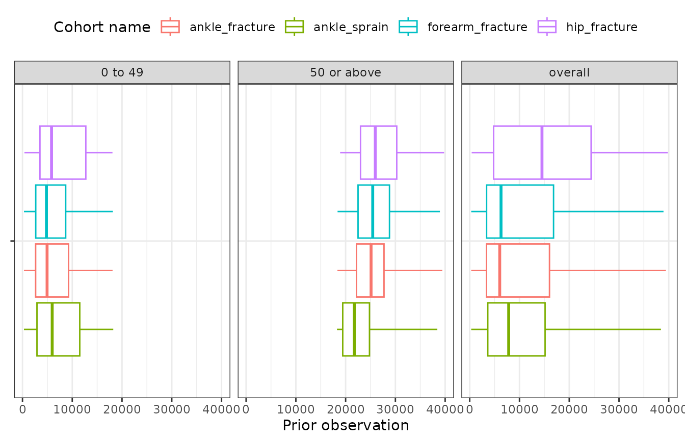
Summaries including presence in other cohorts
We explored whether patients had any exposure to a list of selected medications (acetaminophen, morphine, warfarin)
medsCs <- getDrugIngredientCodes(
  cdm = cdm,
  name = c("acetaminophen", "morphine", "warfarin")
)
cdm <- generateConceptCohortSet(
  cdm = cdm,
  name = "meds",
  conceptSet = medsCs,
  end = "event_end_date",
  limit = "all",
  overwrite = TRUE
)
We can use the intersects arguement inside the function
to get this information.
chars <- cdm$injuries |>
  summariseCharacteristics(cohortIntersectFlag = list(
    "Medications prior to index date" = list(
      targetCohortTable = "meds",
      window = c(-Inf, -1)
    ),
    "Medications on index date" = list(
      targetCohortTable = "meds",
      window = c(0, 0)
    )
  ))
To view the summary table
tableCharacteristics(chars)|
CDM name
|
||||||
|---|---|---|---|---|---|---|
|
GiBleed
|
||||||
| Variable name | Variable level | Estimate name |
Cohort name
|
|||
| ankle_sprain | ankle_fracture | forearm_fracture | hip_fracture | |||
| Number records | – | N | 1,915 | 464 | 569 | 138 |
| Number subjects | – | N | 1,357 | 427 | 510 | 132 |
| Cohort start date | – | Median [Q25 - Q75] | 1982-11-09 [1968-06-15 - 1999-04-13] | 1981-01-15 [1965-03-11 - 1997-08-03] | 1981-07-24 [1967-03-05 - 2000-12-16] | 1996-09-17 [1977-09-20 - 2010-06-22] |
| Range | 1912-02-25 to 2019-05-30 | 1911-09-07 to 2019-06-23 | 1917-08-16 to 2019-06-26 | 1927-12-14 to 2019-05-08 | ||
| Cohort end date | – | Median [Q25 - Q75] | 1982-12-10 [1968-07-06 - 1999-05-09] | 1981-02-28 [1965-04-11 - 1997-10-12] | 1981-08-23 [1967-04-10 - 2001-02-27] | 1996-11-16 [1977-12-04 - 2010-07-22] |
| Range | 1912-03-10 to 2019-05-30 | 1911-12-06 to 2019-06-24 | 1917-11-14 to 2019-06-26 | 1928-03-13 to 2019-06-07 | ||
| Age | – | Median [Q25 - Q75] | 21 [9 - 41] | 16 [9 - 43] | 17 [9 - 46] | 40 [13 - 66] |
| Mean (SD) | 26.63 (21.03) | 27.38 (24.70) | 28.69 (25.97) | 40.06 (28.82) | ||
| Range | 0 to 105 | 0 to 107 | 0 to 106 | 1 to 108 | ||
| Sex | Female | N (%) | 954 (49.82%) | 238 (51.29%) | 286 (50.26%) | 74 (53.62%) |
| Male | N (%) | 961 (50.18%) | 226 (48.71%) | 283 (49.74%) | 64 (46.38%) | |
| Prior observation | – | Median [Q25 - Q75] | 7,833 [3,628 - 15,147] | 6,030 [3,360 - 16,032] | 6,289 [3,390 - 16,847] | 14,522 [4,801 - 24,401] |
| Mean (SD) | 9,918.17 (7,672.74) | 10,196.57 (9,011.31) | 10,670.43 (9,480.30) | 14,821.73 (10,521.89) | ||
| Range | 299 to 38,429 | 299 to 39,430 | 299 to 38,943 | 390 to 39,792 | ||
| Future observation | – | Median [Q25 - Q75] | 12,868 [6,860 - 18,078] | 13,748 [6,878 - 19,331] | 13,165 [5,988 - 18,548] | 7,798 [2,874 - 14,913] |
| Mean (SD) | 12,865.11 (7,543.50) | 13,470.92 (8,215.96) | 12,913.27 (7,929.17) | 9,167.33 (7,160.81) | ||
| Range | 0 to 38,403 | 1 to 39,051 | 0 to 36,654 | 0 to 29,045 | ||
| Days in cohort | – | Median [Q25 - Q75] | 22 [15 - 29] | 61 [31 - 91] | 61 [31 - 91] | 61 [31 - 91] |
| Mean (SD) | 25.02 (8.00) | 61.65 (25.38) | 62.16 (25.32) | 59.26 (24.79) | ||
| Range | 1 to 37 | 2 to 92 | 1 to 91 | 1 to 91 | ||
| Days to next record | – | Median [Q25 - Q75] | 6,082 [2,640 - 10,540] | 5,100 [2,430 - 11,474] | 5,760 [1,922 - 15,606] | 7,430 [2,355 - 15,966] |
| Mean (SD) | 7,457.56 (5,937.15) | 7,784.46 (7,686.21) | 9,217.83 (8,826.17) | 9,037.50 (8,138.51) | ||
| Range | 300 to 29,145 | 330 to 28,365 | 360 to 34,482 | 690 to 19,200 | ||
| Medications prior to index date | 161 acetaminophen | N (%) | 1,530 (79.90%) | 357 (76.94%) | 447 (78.56%) | 119 (86.23%) |
| 11289 warfarin | N (%) | 12 (0.63%) | 8 (1.72%) | 11 (1.93%) | 4 (2.90%) | |
| 7052 morphine | N (%) | 15 (0.78%) | 1 (0.22%) | 2 (0.35%) | 2 (1.45%) | |
| Medications on index date | 161 acetaminophen | N (%) | 773 (40.37%) | 240 (51.72%) | 264 (46.40%) | 90 (65.22%) |
| 11289 warfarin | N (%) | 0 (0.00%) | 0 (0.00%) | 0 (0.00%) | 0 (0.00%) | |
| 7052 morphine | N (%) | 0 (0.00%) | 0 (0.00%) | 0 (0.00%) | 0 (0.00%) | |
To visualise the exposure of these drugs in a bar plot.
plot_data <- chars |>
  filter(
    variable_name == "Medications prior to index date",
    estimate_name == "percentage"
  )

plot_data |>
  plotCharacteristics(
    plotType = "barplot",
    colour = "variable_level",
    facet = c("cdm_name", "cohort_name")
  ) +
  scale_x_discrete(limits = rev(sort(unique(plot_data$variable_level)))) +
  coord_flip() +
  ggtitle("Medication use prior to index date")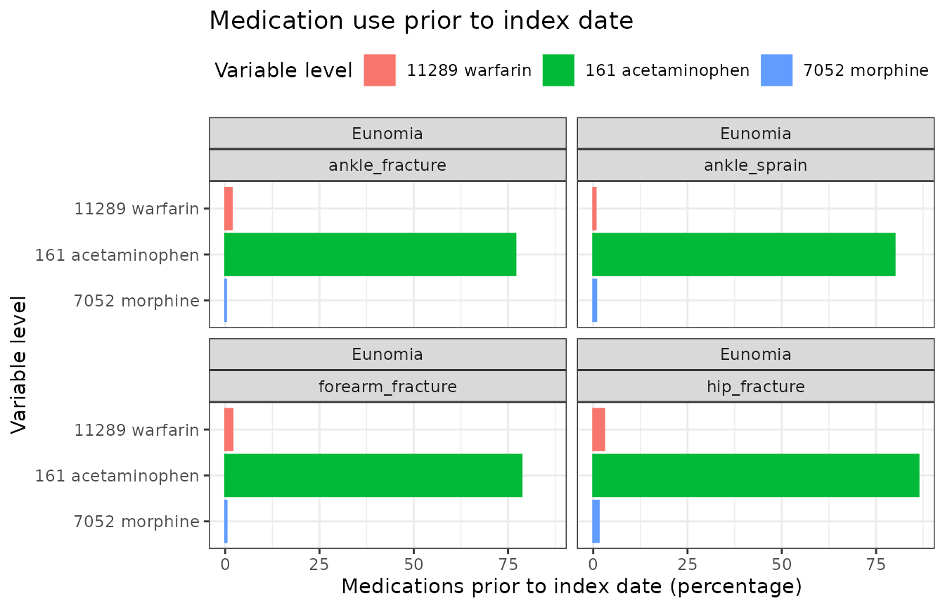
Summaries Using Concept Sets Directly
Instead of creating cohorts, we could have directly used our concept sets for medications when characterising our study cohorts.
chars <- cdm$injuries |>
  summariseCharacteristics(conceptIntersectFlag = list(
    "Medications prior to index date" = list(
      conceptSet = medsCs,
      window = c(-Inf, -1)
    ),
    "Medications on index date" = list(
      conceptSet = medsCs,
      window = c(0, 0)
    )
  ))
Although, like here, concept sets can lead to the same result as using cohorts it is important to note this will not always be the case. This is because the creation of cohorts will have involved the collapsing of overlapping records as well as imposing certain requirements, such as only including records that were observed during an an ongoing observation period. Meanwhile, when working with concept sets we will instead be working directly with record-level data.
tableCharacteristics(chars)|
CDM name
|
||||||
|---|---|---|---|---|---|---|
|
GiBleed
|
||||||
| Variable name | Variable level | Estimate name |
Cohort name
|
|||
| ankle_sprain | ankle_fracture | forearm_fracture | hip_fracture | |||
| Number records | – | N | 1,915 | 464 | 569 | 138 |
| Number subjects | – | N | 1,357 | 427 | 510 | 132 |
| Cohort start date | – | Median [Q25 - Q75] | 1982-11-09 [1968-06-15 - 1999-04-13] | 1981-01-15 [1965-03-11 - 1997-08-03] | 1981-07-24 [1967-03-05 - 2000-12-16] | 1996-09-17 [1977-09-20 - 2010-06-22] |
| Range | 1912-02-25 to 2019-05-30 | 1911-09-07 to 2019-06-23 | 1917-08-16 to 2019-06-26 | 1927-12-14 to 2019-05-08 | ||
| Cohort end date | – | Median [Q25 - Q75] | 1982-12-10 [1968-07-06 - 1999-05-09] | 1981-02-28 [1965-04-11 - 1997-10-12] | 1981-08-23 [1967-04-10 - 2001-02-27] | 1996-11-16 [1977-12-04 - 2010-07-22] |
| Range | 1912-03-10 to 2019-05-30 | 1911-12-06 to 2019-06-24 | 1917-11-14 to 2019-06-26 | 1928-03-13 to 2019-06-07 | ||
| Age | – | Median [Q25 - Q75] | 21 [9 - 41] | 16 [9 - 43] | 17 [9 - 46] | 40 [13 - 66] |
| Mean (SD) | 26.63 (21.03) | 27.38 (24.70) | 28.69 (25.97) | 40.06 (28.82) | ||
| Range | 0 to 105 | 0 to 107 | 0 to 106 | 1 to 108 | ||
| Sex | Female | N (%) | 954 (49.82%) | 238 (51.29%) | 286 (50.26%) | 74 (53.62%) |
| Male | N (%) | 961 (50.18%) | 226 (48.71%) | 283 (49.74%) | 64 (46.38%) | |
| Prior observation | – | Median [Q25 - Q75] | 7,833 [3,628 - 15,147] | 6,030 [3,360 - 16,032] | 6,289 [3,390 - 16,847] | 14,522 [4,801 - 24,401] |
| Mean (SD) | 9,918.17 (7,672.74) | 10,196.57 (9,011.31) | 10,670.43 (9,480.30) | 14,821.73 (10,521.89) | ||
| Range | 299 to 38,429 | 299 to 39,430 | 299 to 38,943 | 390 to 39,792 | ||
| Future observation | – | Median [Q25 - Q75] | 12,868 [6,860 - 18,078] | 13,748 [6,878 - 19,331] | 13,165 [5,988 - 18,548] | 7,798 [2,874 - 14,913] |
| Mean (SD) | 12,865.11 (7,543.50) | 13,470.92 (8,215.96) | 12,913.27 (7,929.17) | 9,167.33 (7,160.81) | ||
| Range | 0 to 38,403 | 1 to 39,051 | 0 to 36,654 | 0 to 29,045 | ||
| Days in cohort | – | Median [Q25 - Q75] | 22 [15 - 29] | 61 [31 - 91] | 61 [31 - 91] | 61 [31 - 91] |
| Mean (SD) | 25.02 (8.00) | 61.65 (25.38) | 62.16 (25.32) | 59.26 (24.79) | ||
| Range | 1 to 37 | 2 to 92 | 1 to 91 | 1 to 91 | ||
| Days to next record | – | Median [Q25 - Q75] | 6,082 [2,640 - 10,540] | 5,100 [2,430 - 11,474] | 5,760 [1,922 - 15,606] | 7,430 [2,355 - 15,966] |
| Mean (SD) | 7,457.56 (5,937.15) | 7,784.46 (7,686.21) | 9,217.83 (8,826.17) | 9,037.50 (8,138.51) | ||
| Range | 300 to 29,145 | 330 to 28,365 | 360 to 34,482 | 690 to 19,200 | ||
| Medications prior to index date | 11289 warfarin | N (%) | 12 (0.63%) | 8 (1.72%) | 11 (1.93%) | 4 (2.90%) |
| 161 acetaminophen | N (%) | 1,530 (79.90%) | 357 (76.94%) | 447 (78.56%) | 119 (86.23%) | |
| 7052 morphine | N (%) | 15 (0.78%) | 1 (0.22%) | 2 (0.35%) | 2 (1.45%) | |
| Medications on index date | 161 acetaminophen | N (%) | 773 (40.37%) | 240 (51.72%) | 264 (46.40%) | 90 (65.22%) |
| 11289 warfarin | N (%) | 0 (0.00%) | 0 (0.00%) | 0 (0.00%) | 0 (0.00%) | |
| 7052 morphine | N (%) | 0 (0.00%) | 0 (0.00%) | 0 (0.00%) | 0 (0.00%) | |
Summaries using clinical tables
More generally, we can also include summaries of the patients’ presence in other clinical tables of the OMOP CDM. For example, here we add a count of visit occurrences
chars <- cdm$injuries |>
  summariseCharacteristics(
    tableIntersectCount = list(
      "Visits in the year prior" = list(
        tableName = "visit_occurrence",
        window = c(-365, -1)
      )
    ),
    tableIntersectFlag = list(
      "Any drug exposure in the year prior" = list(
        tableName = "drug_exposure",
        window = c(-365, -1)
      ),
      "Any procedure in the year prior" = list(
        tableName = "procedure_occurrence",
        window = c(-365, -1)
      )
    )
  )
tableCharacteristics(chars)|
CDM name
|
||||||
|---|---|---|---|---|---|---|
|
GiBleed
|
||||||
| Variable name | Variable level | Estimate name |
Cohort name
|
|||
| ankle_sprain | ankle_fracture | forearm_fracture | hip_fracture | |||
| Number records | – | N | 1,915 | 464 | 569 | 138 |
| Number subjects | – | N | 1,357 | 427 | 510 | 132 |
| Cohort start date | – | Median [Q25 - Q75] | 1982-11-09 [1968-06-15 - 1999-04-13] | 1981-01-15 [1965-03-11 - 1997-08-03] | 1981-07-24 [1967-03-05 - 2000-12-16] | 1996-09-17 [1977-09-20 - 2010-06-22] |
| Range | 1912-02-25 to 2019-05-30 | 1911-09-07 to 2019-06-23 | 1917-08-16 to 2019-06-26 | 1927-12-14 to 2019-05-08 | ||
| Cohort end date | – | Median [Q25 - Q75] | 1982-12-10 [1968-07-06 - 1999-05-09] | 1981-02-28 [1965-04-11 - 1997-10-12] | 1981-08-23 [1967-04-10 - 2001-02-27] | 1996-11-16 [1977-12-04 - 2010-07-22] |
| Range | 1912-03-10 to 2019-05-30 | 1911-12-06 to 2019-06-24 | 1917-11-14 to 2019-06-26 | 1928-03-13 to 2019-06-07 | ||
| Age | – | Median [Q25 - Q75] | 21 [9 - 41] | 16 [9 - 43] | 17 [9 - 46] | 40 [13 - 66] |
| Mean (SD) | 26.63 (21.03) | 27.38 (24.70) | 28.69 (25.97) | 40.06 (28.82) | ||
| Range | 0 to 105 | 0 to 107 | 0 to 106 | 1 to 108 | ||
| Sex | Female | N (%) | 954 (49.82%) | 238 (51.29%) | 286 (50.26%) | 74 (53.62%) |
| Male | N (%) | 961 (50.18%) | 226 (48.71%) | 283 (49.74%) | 64 (46.38%) | |
| Prior observation | – | Median [Q25 - Q75] | 7,833 [3,628 - 15,147] | 6,030 [3,360 - 16,032] | 6,289 [3,390 - 16,847] | 14,522 [4,801 - 24,401] |
| Mean (SD) | 9,918.17 (7,672.74) | 10,196.57 (9,011.31) | 10,670.43 (9,480.30) | 14,821.73 (10,521.89) | ||
| Range | 299 to 38,429 | 299 to 39,430 | 299 to 38,943 | 390 to 39,792 | ||
| Future observation | – | Median [Q25 - Q75] | 12,868 [6,860 - 18,078] | 13,748 [6,878 - 19,331] | 13,165 [5,988 - 18,548] | 7,798 [2,874 - 14,913] |
| Mean (SD) | 12,865.11 (7,543.50) | 13,470.92 (8,215.96) | 12,913.27 (7,929.17) | 9,167.33 (7,160.81) | ||
| Range | 0 to 38,403 | 1 to 39,051 | 0 to 36,654 | 0 to 29,045 | ||
| Days in cohort | – | Median [Q25 - Q75] | 22 [15 - 29] | 61 [31 - 91] | 61 [31 - 91] | 61 [31 - 91] |
| Mean (SD) | 25.02 (8.00) | 61.65 (25.38) | 62.16 (25.32) | 59.26 (24.79) | ||
| Range | 1 to 37 | 2 to 92 | 1 to 91 | 1 to 91 | ||
| Days to next record | – | Median [Q25 - Q75] | 6,082 [2,640 - 10,540] | 5,100 [2,430 - 11,474] | 5,760 [1,922 - 15,606] | 7,430 [2,355 - 15,966] |
| Mean (SD) | 7,457.56 (5,937.15) | 7,784.46 (7,686.21) | 9,217.83 (8,826.17) | 9,037.50 (8,138.51) | ||
| Range | 300 to 29,145 | 330 to 28,365 | 360 to 34,482 | 690 to 19,200 | ||
| Any drug exposure in the year prior | – | N (%) | 597 (31.17%) | 149 (32.11%) | 171 (30.05%) | 41 (29.71%) |
| Any procedure in the year prior | – | N (%) | 123 (6.42%) | 26 (5.60%) | 37 (6.50%) | 15 (10.87%) |
| Visits in the year prior | – | Median [Q25 - Q75] | 0.00 [0.00 - 0.00] | 0.00 [0.00 - 0.00] | 0.00 [0.00 - 0.00] | 0.00 [0.00 - 0.00] |
| Mean (SD) | 0.00 (0.06) | 0.00 (0.00) | 0.00 (0.00) | 0.00 (0.00) | ||
| Range | 0.00 to 1.00 | 0.00 to 0.00 | 0.00 to 0.00 | 0.00 to 0.00 | ||