Estimate Survival from Common Data Model Cohorts • CohortSurvival

CohortSurvival contains functions for extracting and summarising survival data using the OMOP common data model.

Installation

You can install CohortSurvival like so:

install.packages("CohortSurvival")

Example usage

Create a reference to data in the OMOP CDM format

The CohortSurvival package is designed to work with data in the OMOP CDM format, so our first step is to create a reference to the data using the CDMConnector package.

For this example we´ll use a cdm reference containing the MGUS2 dataset from the survival package (which we transformed into a set of OMOP CDM style cohort tables). The MGUS2 dataset contains survival data of 1341 sequential patients with monoclonal gammopathy of undetermined significance (MGUS). For more information see ?survival::mgus2.

library(CDMConnector)
library(CohortSurvival)
library(dplyr)
library(ggplot2)

cdm <- CohortSurvival::mockMGUS2cdm()

In our cdm reference we have three cohort tables of interest: 1) MGUS diagnosis cohort

cdm$mgus_diagnosis %>%
  glimpse()
#> Rows: ??
#> Columns: 10
#> Database: DuckDB v1.1.3 [lopezk@Windows 10 x64:R 4.3.2/:memory:]
#> $ cohort_definition_id <int> 1, 1, 1, 1, 1, 1, 1, 1, 1, 1, 1, 1, 1, 1, 1, 1, 1…
#> $ subject_id           <int> 1, 2, 3, 4, 5, 6, 7, 8, 9, 10, 11, 12, 13, 14, 15…
#> $ cohort_start_date    <date> 1981-01-01, 1968-01-01, 1980-01-01, 1977-01-01, …
#> $ cohort_end_date      <date> 1981-01-01, 1968-01-01, 1980-01-01, 1977-01-01, …
#> $ age                  <dbl> 88, 78, 94, 68, 90, 90, 89, 87, 86, 79, 86, 89, 8…
#> $ sex                  <fct> F, F, M, M, F, M, F, F, F, F, M, F, M, F, M, F, F…
#> $ hgb                  <dbl> 13.1, 11.5, 10.5, 15.2, 10.7, 12.9, 10.5, 12.3, 1…
#> $ creat                <dbl> 1.30, 1.20, 1.50, 1.20, 0.80, 1.00, 0.90, 1.20, 0…
#> $ mspike               <dbl> 0.5, 2.0, 2.6, 1.2, 1.0, 0.5, 1.3, 1.6, 2.4, 2.3,…
#> $ age_group            <chr> ">=70", ">=70", ">=70", "<70", ">=70", ">=70", ">…

MGUS progression to multiple myeloma cohort

cdm$progression %>%
  glimpse()
#> Rows: ??
#> Columns: 4
#> Database: DuckDB v1.1.3 [lopezk@Windows 10 x64:R 4.3.2/:memory:]
#> $ cohort_definition_id <int> 1, 1, 1, 1, 1, 1, 1, 1, 1, 1, 1, 1, 1, 1, 1, 1, 1…
#> $ subject_id           <int> 56, 81, 83, 111, 124, 127, 147, 163, 165, 167, 18…
#> $ cohort_start_date    <date> 1978-01-30, 1985-01-15, 1974-08-17, 1993-01-14, …
#> $ cohort_end_date      <date> 1978-01-30, 1985-01-15, 1974-08-17, 1993-01-14, …

Death cohort

cdm$death_cohort %>%
  glimpse()
#> Rows: ??
#> Columns: 4
#> Database: DuckDB v1.1.3 [lopezk@Windows 10 x64:R 4.3.2/:memory:]
#> $ cohort_definition_id <int> 1, 1, 1, 1, 1, 1, 1, 1, 1, 1, 1, 1, 1, 1, 1, 1, 1…
#> $ subject_id           <int> 1, 2, 3, 4, 5, 6, 7, 8, 10, 11, 12, 13, 14, 15, 1…
#> $ cohort_start_date    <date> 1981-01-31, 1968-01-26, 1980-02-16, 1977-04-03, …
#> $ cohort_end_date      <date> 1981-01-31, 1968-01-26, 1980-02-16, 1977-04-03, …

MGUS diagnosis to death

We can get survival estimates for death following MGUS diagnosis like so:

MGUS_death <- estimateSingleEventSurvival(cdm,
  targetCohortTable = "mgus_diagnosis",
  outcomeCohortTable = "death_cohort"
)
MGUS_death %>% 
  glimpse()
#> Rows: 1,354
#> Columns: 13
#> $ result_id        <int> 1, 1, 1, 1, 1, 1, 1, 1, 1, 1, 1, 1, 1, 1, 1, 1, 1, 1,…
#> $ cdm_name         <chr> "mock", "mock", "mock", "mock", "mock", "mock", "mock…
#> $ group_name       <chr> "target_cohort", "target_cohort", "target_cohort", "t…
#> $ group_level      <chr> "mgus_diagnosis", "mgus_diagnosis", "mgus_diagnosis",…
#> $ strata_name      <chr> "overall", "overall", "overall", "overall", "overall"…
#> $ strata_level     <chr> "overall", "overall", "overall", "overall", "overall"…
#> $ variable_name    <chr> "outcome", "outcome", "outcome", "outcome", "outcome"…
#> $ variable_level   <chr> "death_cohort", "death_cohort", "death_cohort", "deat…
#> $ estimate_name    <chr> "estimate", "estimate_95CI_lower", "estimate_95CI_upp…
#> $ estimate_type    <chr> "numeric", "numeric", "numeric", "numeric", "numeric"…
#> $ estimate_value   <chr> "1", "1", "1", "0.9697", "0.9607", "0.9787", "0.9494"…
#> $ additional_name  <chr> "time", "time", "time", "time", "time", "time", "time…
#> $ additional_level <chr> "0", "0", "0", "1", "1", "1", "2", "2", "2", "3", "3"…

Now that we have our results, we can quickly create a plot summarising survival over time.

plotSurvival(MGUS_death)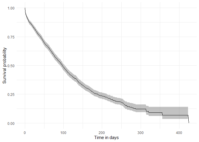

Among others, we can check the survival summary of our target and outcome cohorts of interest:

tableSurvival(MGUS_death, times = c(30,60,180))

CDM name	Target cohort	Outcome name	Estimate name
CDM name	Target cohort	Outcome name	Number records	Number events	Median survival (95% CI)	Restricted mean survival (SE)	30 days survival estimate	60 days survival estimate	180 days survival estimate
mock	mgus_diagnosis	death_cohort	1,384	963	98.00 (92.00, 103.00)	133.00 (4.00)	79.39 (77.28, 81.55)	66.15 (63.70, 68.70)	25.90 (23.35, 28.72)

As well as estimating survival for our cohort overall, we can also estimate survival by strata. These strata are based on variables that have been added to our target cohort previously as columns.

MGUS_death <- estimateSingleEventSurvival(cdm,
  targetCohortTable = "mgus_diagnosis",
  outcomeCohortTable = "death_cohort",
  strata = list(c("age_group"),
                c("sex"),
                c("age_group", "sex"))
)

plotSurvival(MGUS_death, 
             colour = "strata_level", 
             facet= "strata_name")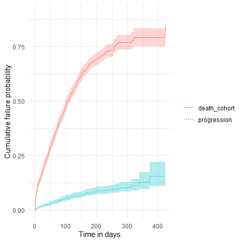

Estimating survival accounting for a competing risk

The package also allows to estimate survival of both an outcome and competing risk outcome together. We can then stratify, see information on events or summarise the estimates in the same way we did for the single event survival analysis.

MGUS_death_prog <- estimateCompetingRiskSurvival(cdm,
  targetCohortTable = "mgus_diagnosis",
  outcomeCohortTable = "progression",
  competingOutcomeCohortTable = "death_cohort"
)

plotSurvival(MGUS_death_prog, cumulativeFailure = TRUE,
             colour = "variable_level")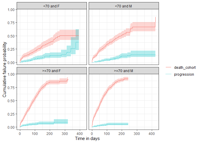

As with single event survival, we can stratify our competing risk analysis.

MGUS_death_prog <-  estimateCompetingRiskSurvival(cdm,
  targetCohortTable = "mgus_diagnosis",
  outcomeCohortTable = "progression",
  competingOutcomeCohortTable = "death_cohort",
  strata = list(c("age_group", "sex"))
)

plotSurvival(MGUS_death_prog  %>%
             dplyr::filter(strata_name != "overall"), 
             cumulativeFailure = TRUE,
             facet = "strata_level",
             colour = "variable_level")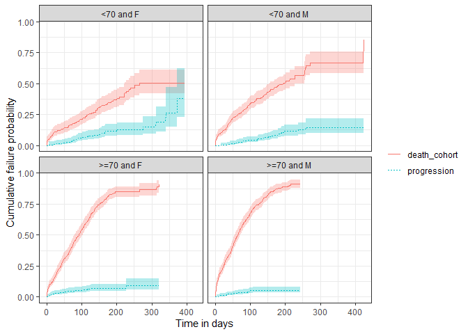

Disconnect from the cdm database connection

cdmDisconnect(cdm)

Additional information

You can check additional functionality of the package on its website.