Tables and figures • ReportGenerator

DISEASE EPIDEMIOLOGY

Population-level descriptive epidemiology

These analyses include an assessment of the incidence or prevalence of specific conditions, eventually stratified by time or by population subgroups like age or sex.

A typical population-level descriptive epidemiology study will have an objective like:

To estimate the monthly incidence rate and point prevalence of disease A stratified by sex and age.

Report Contents

The report will include an executive summary and the following tables and figures:

Table 1: Number of participants and total number of incident and/or prevalent cases in each data source during the study period. Number of participants per pre-specified strata will be included where necessary/applicable.

CohortCharacteristics::tableCharacteristics(
  result,
  type = "gt",
  header = c("cdm_name", "cohort_name"),
  groupColumn = character(),
  hide = c(additionalColumns(result), settingsColumns(result)),
  .options = list(style = "darwin")
)

			CDM name
			PP_MOCK
Variable name	Variable level	Estimate name	Cohort name
Variable name	Variable level	Estimate name	cohort_1	cohort_2	cohort_3
Number records	-	N	6	2	2
Number subjects	-	N	6	2	2
Cohort start date	-	Median [Q25 - Q75]	1976-02-17 [1926-12-14 - 1983-07-28]	1955-12-29 [1943-09-07 - 1968-04-20]	1991-04-01 [1980-01-29 - 2002-06-01]
		Range	1907-01-04 to 1991-11-21	1931-05-17 to 1980-08-11	1968-11-27 to 2013-08-02
Cohort end date	-	Median [Q25 - Q75]	1983-05-14 [1930-11-19 - 1990-08-18]	1958-08-28 [1945-02-08 - 1972-03-17]	1995-05-06 [1986-03-13 - 2004-06-27]
		Range	1912-07-22 to 1997-10-31	1931-07-22 to 1985-10-05	1977-01-19 to 2013-08-19
Age	-	Median [Q25 - Q75]	7 [3 - 18]	12 [10 - 15]	24 [19 - 30]
		Mean (SD)	12.17 (12.59)	12.50 (7.78)	24.50 (16.26)
		Range	2 to 33	7 to 18	13 to 36
Sex	Female	N (%)	4 (66.67%)	2 (100.00%)	1 (50.00%)
	Male	N (%)	2 (33.33%)	-	1 (50.00%)
Prior observation	-	Median [Q25 - Q75]	2,850 [1,354 - 7,065]	4,745 [3,719 - 5,771]	9,220 [7,150 - 11,291]
		Mean (SD)	4,672.67 (4,637.15)	4,745.00 (2,901.97)	9,220.50 (5,856.97)
		Range	733 to 12,276	2,693 to 6,797	5,079 to 13,362
Future observation	-	Median [Q25 - Q75]	7,254 [4,476 - 12,970]	2,052 [1,789 - 2,314]	3,466 [2,248 - 4,685]
		Mean (SD)	8,389.17 (5,498.88)	2,051.50 (743.17)	3,466.50 (3,447.15)
		Range	2,246 to 15,156	1,526 to 2,577	1,029 to 5,904
Days in cohort	-	Median [Q25 - Q75]	2,366 [2,063 - 2,578]	974 [521 - 1,428]	1,497 [758 - 2,236]
		Mean (SD)	2,179.50 (633.44)	974.50 (1,283.40)	1,497.00 (2,091.62)
		Range	1,007 to 2,727	67 to 1,882	18 to 2,976

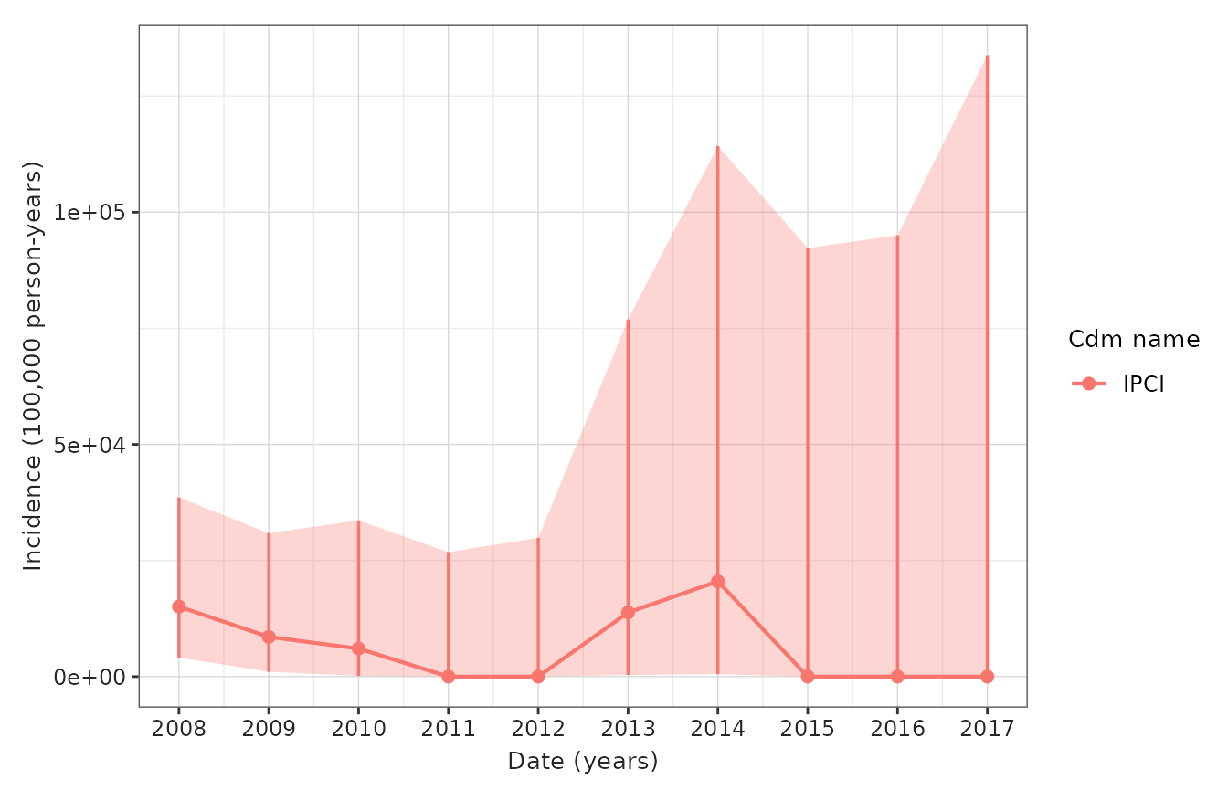
Figure 1: Incidence rate/s of disease over calendar time (per month/year) overall

IncidencePrevalence::plotIncidence(
  result = incidence_result_figure_1,
  x = "incidence_start_date",
  y = "incidence_100000_pys",
  line = TRUE,
  point = TRUE,
  ribbon = TRUE,
  ymin = "incidence_100000_pys_95CI_lower",
  ymax = "incidence_100000_pys_95CI_upper",
  facet = NULL,
  colour = "cdm_name"
)

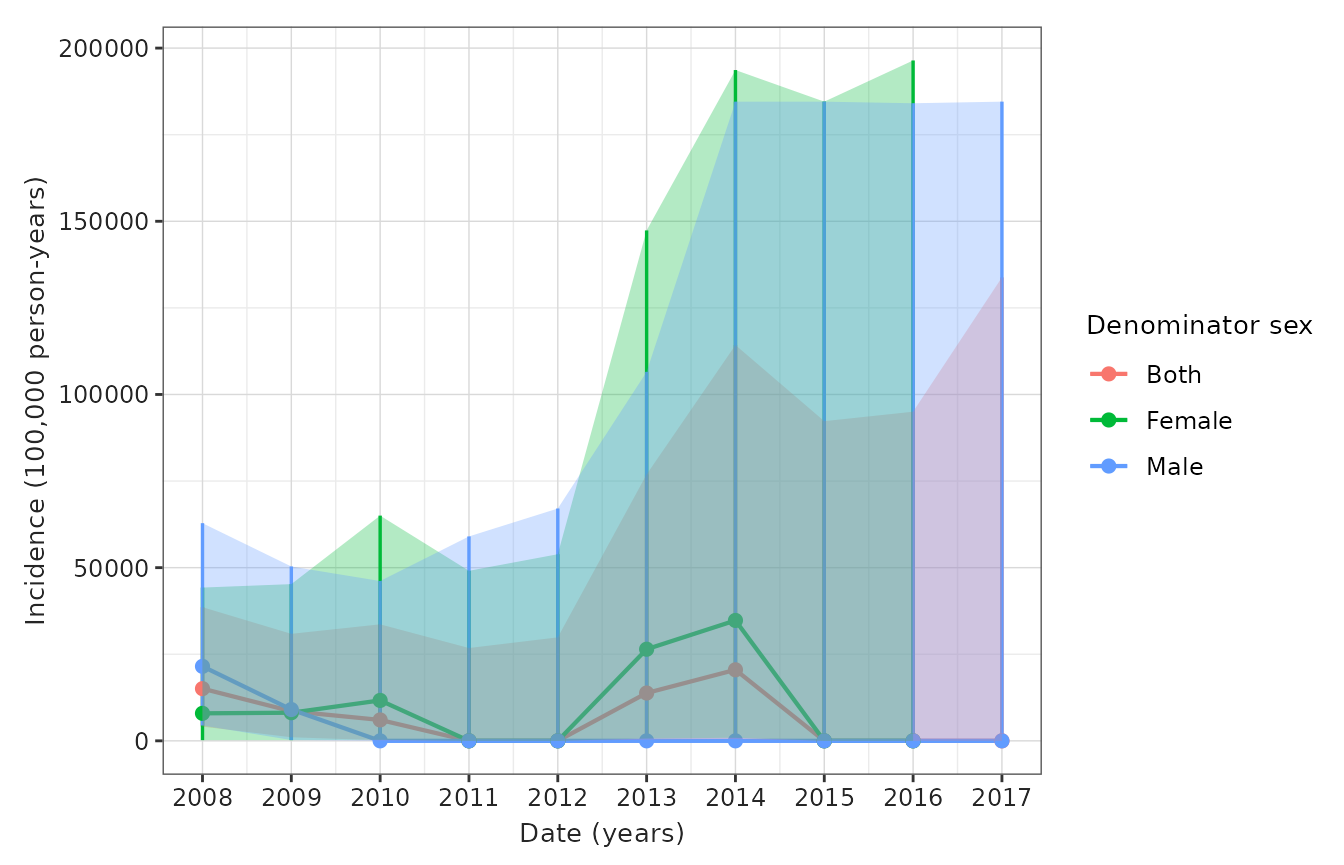
Figure 2: Incidence rate/s of disease over calendar time (per month/year) stratified by sex and age (or other pre-specified criterion/a)

IncidencePrevalence::plotIncidence(
  result = incidence_result_figure_2a,
  x = "incidence_start_date",
  y = "incidence_100000_pys",
  line = TRUE,
  point = TRUE,
  ribbon = TRUE,
  ymin = "incidence_100000_pys_95CI_lower",
  ymax = "incidence_100000_pys_95CI_upper",
  facet = NULL,
  colour = "denominator_sex"
)

IncidencePrevalence::plotIncidence(
  result = incidence_result_figure_2b,
  x = "incidence_start_date",
  y = "incidence_100000_pys",
  line = TRUE,
  point = TRUE,
  ribbon = TRUE,
  ymin = "incidence_100000_pys_95CI_lower",
  ymax = "incidence_100000_pys_95CI_upper",
  facet = NULL,
  colour = "denominator_age_group"
)

Table 2: Numbers reported in figures 1 and 2

IncidencePrevalence::tableIncidence(
  result = incidence_result_table_2,
  type = "gt",
  header = c("estimate_name"),
  groupColumn = c("cdm_name", "outcome_cohort_name"),
  settingsColumn = c("denominator_age_group", "denominator_sex"),
  hide = c("denominator_cohort_name", "analysis_interval"),
  .options = list(style = "darwin")
)

Incidence start date	Incidence end date	Denominator age group	Denominator sex	Estimate name
Incidence start date	Incidence end date	Denominator age group	Denominator sex	Denominator (N)	Person-years	Outcome (N)	Incidence 100,000 person-years [95% CI]
IPCI; cohort_1
2008-01-01	2008-12-31	0 to 64	Both	32	26.54	4	15,069.89 (4,106.04 - 38,584.89)
2009-01-01	2009-12-31	0 to 64	Both	30	23.38	2	8,552.86 (1,035.79 - 30,895.86)
2010-01-01	2010-12-31	0 to 64	Both	22	16.56	1	6,037.19 (152.85 - 33,637.07)
2011-01-01	2011-12-31	0 to 64	Both	16	13.77	0	0.00 (0.00 - 26,797.03)
2012-01-01	2012-12-31	0 to 64	Both	13	12.35	0	0.00 (0.00 - 29,874.31)
2013-01-01	2013-12-31	0 to 64	Both	11	7.24	1	13,804.53 (349.50 - 76,913.91)
2014-01-01	2014-12-31	0 to 64	Both	5	4.88	1	20,508.61 (519.23 - 114,266.68)
2015-01-01	2015-12-31	0 to 64	Both	4	4.00	0	0.00 (0.00 - 92,291.20)
2016-01-01	2016-12-31	0 to 64	Both	5	3.88	0	0.00 (0.00 - 95,025.23)
2017-01-01	2017-12-31	0 to 64	Both	3	2.76	0	0.00 (0.00 - 133,800.49)

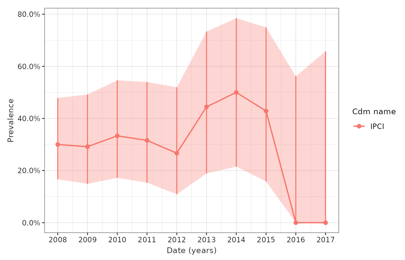
Figure 3: Prevalence of disease over calendar time (per month/year) overall

IncidencePrevalence::plotPrevalence(
  result = prevalence_result_figure_1,
  x = "prevalence_start_date",
  y = "prevalence",
  line = TRUE,
  point = TRUE,
  ribbon = TRUE,
  ymin = "prevalence_95CI_lower",
  ymax = "prevalence_95CI_upper",
  facet = NULL,
  colour = "cdm_name"
)

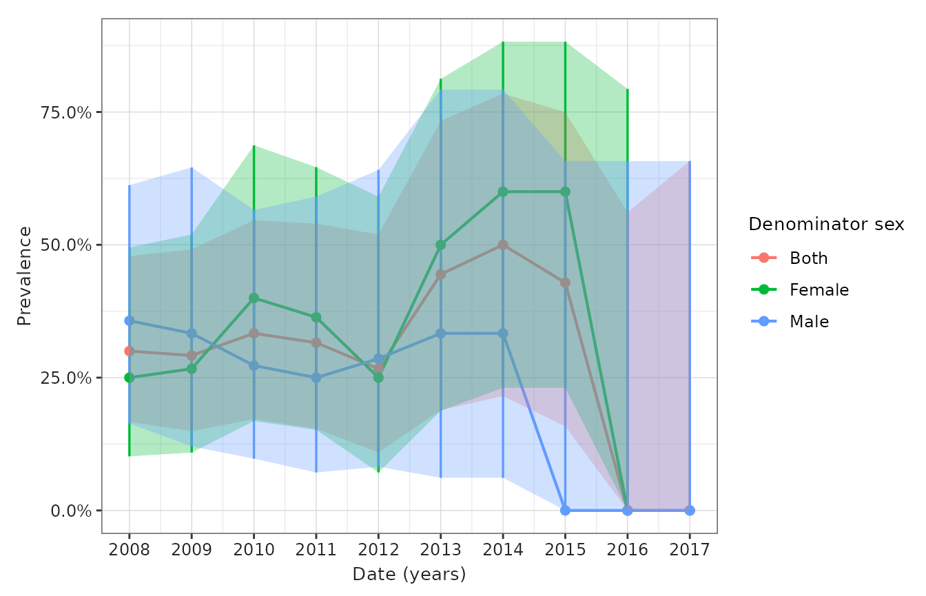
Figure 4: Prevalence of disease over calendar time (per month/year) stratified by sex and age (or other pre-specified criterion/a)

IncidencePrevalence::plotPrevalence(
  result = prevalence_result_figure_2a,
  x = "prevalence_start_date",
  y = "prevalence",
  line = TRUE,
  point = TRUE,
  ribbon = TRUE,
  ymin = "prevalence_95CI_lower",
  ymax = "prevalence_95CI_upper",
  facet = NULL,
  colour = "denominator_sex"
)

IncidencePrevalence::plotPrevalence(
  result = prevalence_result_figure_2b,
  x = "prevalence_start_date",
  y = "prevalence",
  line = TRUE,
  point = TRUE,
  ribbon = TRUE,
  ymin = "prevalence_95CI_lower",
  ymax = "prevalence_95CI_upper",
  facet = NULL,
  colour = "denominator_age_group"
)

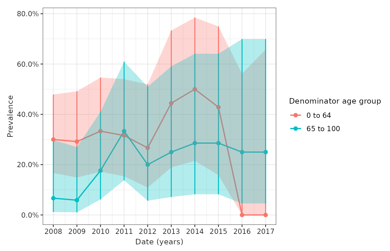
Table 3: Numbers reported in Figures 3 and 4.

IncidencePrevalence::tablePrevalence(
  result = prevalence_result_table_2,
  type = "gt",
  header = c("estimate_name"),
  groupColumn = c("cdm_name", "outcome_cohort_name"),
  settingsColumn = c("denominator_age_group", "denominator_sex"),
  hide = c("denominator_cohort_name", "analysis_interval"),
  .options = list(style = "darwin")
)

Prevalence start date	Prevalence end date	Denominator age group	Denominator sex	Estimate name
Prevalence start date	Prevalence end date	Denominator age group	Denominator sex	Denominator (N)	Outcome (N)	Prevalence [95% CI]
IPCI; cohort_1
2008-01-01	2008-12-31	0 to 64	Both	30	9	0.30 (0.17 - 0.48)
2009-01-01	2009-12-31	0 to 64	Both	24	7	0.29 (0.15 - 0.49)
2010-01-01	2010-12-31	0 to 64	Both	21	7	0.33 (0.17 - 0.55)
2011-01-01	2011-12-31	0 to 64	Both	19	6	0.32 (0.15 - 0.54)
2012-01-01	2012-12-31	0 to 64	Both	15	4	0.27 (0.11 - 0.52)
2013-01-01	2013-12-31	0 to 64	Both	9	4	0.44 (0.19 - 0.73)
2014-01-01	2014-12-31	0 to 64	Both	8	4	0.50 (0.22 - 0.78)
2015-01-01	2015-12-31	0 to 64	Both	7	3	0.43 (0.16 - 0.75)
2016-01-01	2016-12-31	0 to 64	Both	3	0	0.00 (0.00 - 0.56)
2017-01-01	2017-12-31	0 to 64	Both	2	0	0.00 (0.00 - 0.66)

Patient-level characterization

These analyses include a descriptive analysis of a cohort of patients newly diagnosed with a specific condition of interest. This characterization typically includes pre-specified features (e.g. history of a certain list of diseases) as well as a list of the most commonly recorded codes in the patient records, and can be stratified by age, sex, or other characteristics.

A typical patient-level characterization study will have an objective that reads something like:

To characterise patients newly diagnosed with condition A, including an assessment of age, sex, and previous comorbidities, as well as a descriptive analysis of how they are treated in the year after diagnosis

Report Contents

The report will include an executive summary and the following tables and figures:

Table 1. Pre-index characteristics of patients newly diagnosed with a condition of interest, at the time of diagnosis/recording. Number of participants per pre-specified strata will be included where necessary/applicable.

CohortCharacteristics::tableCharacteristics(
  result = summarise_characteristics,
  type = "gt",
  header = c("cdm_name", "cohort_name"),
  groupColumn = "variable_name",
  hide = c("table", "window", "value", "table_name"),
  .options = list(style = "darwin")
)

		CDM name
		IPCI
Variable level	Estimate name	Cohort name
Variable level	Estimate name	ankle_sprain	ankle_fracture	forearm_fracture	hip_fracture
Number records
-	N	1,915	464	569	138
Number subjects
-	N	1,357	427	510	132
Cohort start date
-	Median [Q25 - Q75]	1982-11-09 [1968-06-15 - 1999-04-13]	1981-01-15 [1965-03-11 - 1997-08-03]	1981-07-24 [1967-03-05 - 2000-12-16]	1996-09-17 [1977-09-20 - 2010-06-22]
	Range	1912-02-25 to 2019-05-30	1911-09-07 to 2019-06-23	1917-08-16 to 2019-06-26	1927-12-14 to 2019-05-08
Cohort end date
-	Median [Q25 - Q75]	1982-12-10 [1968-07-06 - 1999-05-09]	1981-02-28 [1965-04-11 - 1997-10-12]	1981-08-23 [1967-04-10 - 2001-02-27]	1996-11-16 [1977-12-04 - 2010-07-22]
	Range	1912-03-10 to 2019-05-30	1911-12-06 to 2019-06-24	1917-11-14 to 2019-06-26	1928-03-13 to 2019-06-07
Age
-	Median [Q25 - Q75]	21 [9 - 41]	16 [9 - 43]	17 [9 - 46]	40 [13 - 66]
	Mean (SD)	26.63 (21.03)	27.38 (24.70)	28.69 (25.97)	40.06 (28.82)
	Range	0 to 105	0 to 107	0 to 106	1 to 108
Sex
Female	N (%)	954 (49.82%)	238 (51.29%)	286 (50.26%)	74 (53.62%)
Male	N (%)	961 (50.18%)	226 (48.71%)	283 (49.74%)	64 (46.38%)
Prior observation
-	Median [Q25 - Q75]	7,833 [3,628 - 15,147]	6,030 [3,360 - 16,032]	6,289 [3,390 - 16,847]	14,522 [4,801 - 24,401]
	Mean (SD)	9,918.17 (7,672.74)	10,196.57 (9,011.31)	10,670.43 (9,480.30)	14,821.73 (10,521.89)
	Range	299 to 38,429	299 to 39,430	299 to 38,943	390 to 39,792
Future observation
-	Median [Q25 - Q75]	12,868 [6,860 - 18,078]	13,748 [6,878 - 19,331]	13,165 [5,988 - 18,548]	7,798 [2,874 - 14,913]
	Mean (SD)	12,865.11 (7,543.50)	13,470.92 (8,215.96)	12,913.27 (7,929.17)	9,167.33 (7,160.81)
	Range	0 to 38,403	1 to 39,051	0 to 36,654	0 to 29,045
Days in cohort
-	Median [Q25 - Q75]	22 [15 - 29]	61 [31 - 91]	61 [31 - 91]	61 [31 - 91]
	Mean (SD)	25.02 (8.00)	61.65 (25.38)	62.16 (25.32)	59.26 (24.79)
	Range	1 to 37	2 to 92	1 to 91	1 to 91
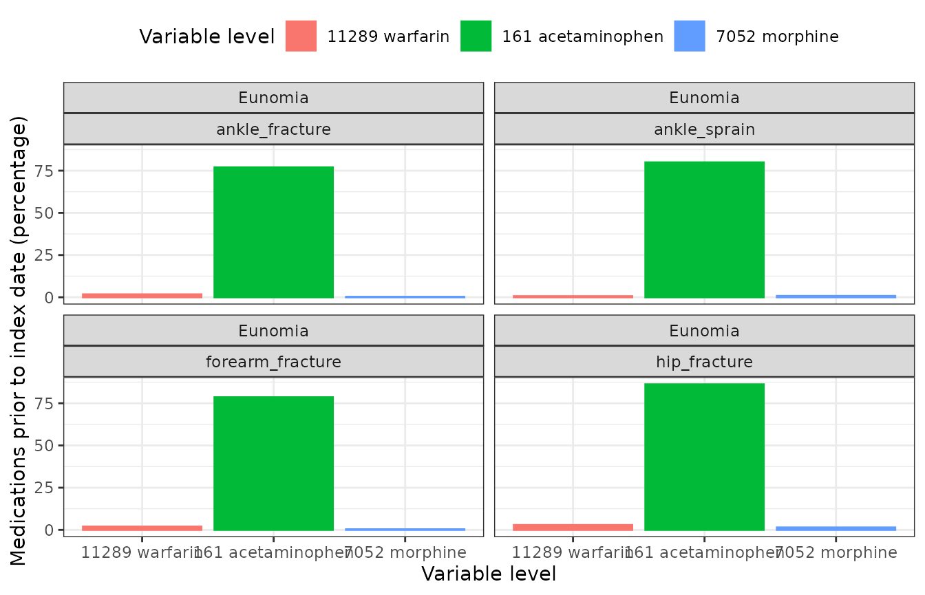
Medications prior to index date
Acetaminophen	N (%)	1,530 (79.90%)	357 (76.94%)	447 (78.56%)	119 (86.23%)
Warfarin	N (%)	12 (0.63%)	8 (1.72%)	11 (1.93%)	4 (2.90%)
Morphine	N (%)	15 (0.78%)	1 (0.22%)	2 (0.35%)	2 (1.45%)
Medications on index date
Acetaminophen	N (%)	773 (40.37%)	240 (51.72%)	264 (46.40%)	90 (65.22%)
Morphine	N (%)	0 (0.00%)	0 (0.00%)	0 (0.00%)	0 (0.00%)
Warfarin	N (%)	0 (0.00%)	0 (0.00%)	0 (0.00%)	0 (0.00%)

Table 2. Number and percentage with an outcome of interest in the x years following diagnosis.

CohortCharacteristics::tableTopLargeScaleCharacteristics(
  result = lsc_characteristics,
  topConcepts = 10,
  type = "gt"
)

	Window
	-inf to -1			0 to 0
	Table name
	condition_occurrence	drug_exposure	procedure_occurrence	condition_occurrence	drug_exposure
Top	Type
Top	event	episode	event	event	episode
1	Viral sinusitis (40481087) 981 (72.3%)	poliovirus vaccine, inactivated (40213160) 994 (73.2%)	Suture open wound (4125906) 363 (26.8%)	Sprain of ankle (81151) 1357 (100.0%)	Aspirin 81 MG Oral Tablet (19059056) 470 (34.6%)
2	Otitis media (372328) 909 (67.0%)	Aspirin 81 MG Oral Tablet (19059056) 842 (62.0%)	Bone immobilization (4170947) 356 (26.2%)		Acetaminophen 325 MG Oral Tablet (1127433) 330 (24.3%)
3	Acute viral pharyngitis (4112343) 845 (62.3%)	Acetaminophen 325 MG Oral Tablet (1127433) 737 (54.3%)	Sputum examination (4151422) 282 (20.8%)		Acetaminophen 160 MG Oral Tablet (1127078) 199 (14.7%)
4	Acute bronchitis (260139) 767 (56.5%)	Acetaminophen 160 MG Oral Tablet (1127078) 559 (41.2%)	Plain chest X-ray (4163872) 137 (10.1%)		Ibuprofen 200 MG Oral Tablet (19078461) 192 (14.2%)
5	Streptococcal sore throat (28060) 499 (36.8%)	Amoxicillin 250 MG / Clavulanate 125 MG Oral Tablet (1713671) 499 (36.8%)
6	Osteoarthritis (80180) 283 (20.9%)	Penicillin V Potassium 250 MG Oral Tablet (19133873) 491 (36.2%)
7	Concussion with no loss of consciousness (378001) 185 (13.6%)	Penicillin G 375 MG/ML Injectable Solution (19006318) 384 (28.3%)
8	Acute bacterial sinusitis (4294548) 168 (12.4%)	Acetaminophen 21.7 MG/ML / Dextromethorphan Hydrobromide 1 MG/ML / doxylamine succinate 0.417 MG/ML Oral Solution (40229134) 296 (21.8%)
9	Sinusitis (4283893) 166 (12.2%)	tetanus and diphtheria toxoids, adsorbed, preservative free, for adult use (40213227) 288 (21.2%)
10	Chronic sinusitis (257012) 162 (11.9%)	hepatitis B vaccine, adult dosage (40213306) 226 (16.6%)

Figure 1. Kaplan-Meier or Cumulative Incidence Function plots of the probability of a pre-specified outcome following index diagnosis of the condition of interest.

CohortSurvival::tableSurvival(
  x = single_event_data,
  times = NULL,
  timeScale = "days",
  header = c("estimate"),
  type = "gt",
  groupColumn = NULL,
  .options = list(style = "darwin")
)

CDM name	Target cohort	Age group	Sex	Outcome name	Estimate name
CDM name	Target cohort	Age group	Sex	Outcome name	Number records	Number events	Median survival (95% CI)	Restricted mean survival (95% CI)
IPCI	mgus_diagnosis	overall	overall	death_cohort	1,384	963	98.00 (92.00, 103.00)	133.00 (124.00, 141.00)
		<70	overall	death_cohort	574	293	180.00 (158.00, 206.00)	197.00 (181.00, 214.00)
		>=70	overall	death_cohort	810	670	71.00 (66.00, 77.00)	86.00 (80.00, 91.00)
		overall	F	death_cohort	631	423	108.00 (100.00, 121.00)	143.00 (131.00, 156.00)
			M	death_cohort	753	540	88.00 (79.00, 97.00)	125.00 (114.00, 136.00)
		<70	F	death_cohort	240	109	215.00 (179.00, 260.00)	220.00 (194.00, 245.00)
			M	death_cohort	334	184	158.00 (139.00, 189.00)	183.00 (163.00, 203.00)
		>=70	F	death_cohort	391	314	82.00 (75.00, 94.00)	96.00 (87.00, 105.00)
			M	death_cohort	419	356	61.00 (54.00, 70.00)	80.00 (71.00, 90.00)

CohortSurvival::riskTable(
  x = competing_risk_data,
  eventGap = NULL,
  header = c("estimate"),
  type = "gt",
  groupColumn = NULL,
  .options = list(style = "darwin")
)

CDM name	Target cohort	Sex	Outcome type	Outcome name	Time	Event gap	Estimate name
CDM name	Target cohort	Sex	Outcome type	Outcome name	Time	Event gap	Number at risk	Number events	Number censored
IPCI	mgus_diagnosis	overall	outcome	progression	0	30	1,384	0	0
					30	30	1,090	25	3
					60	30	874	19	27
					90	30	635	19	77
					120	30	424	13	74
					150	30	288	9	52
					180	30	178	10	52
					210	30	103	4	54
					240	30	57	2	32
					270	30	29	1	18
					300	30	16	1	10
					330	30	7	1	6
					360	30	3	1	3
					390	30	2	1	0
					420	30	1	0	1
					424	30	1	0	0
			competing_outcome	death_cohort	0	30	1,384	0	0
					30	30	1,090	275	3
					60	30	874	170	27
					90	30	635	147	77
					120	30	424	113	74
					150	30	288	77	52
					180	30	178	47	52
					210	30	103	16	54
					240	30	57	12	32
					270	30	29	8	18
					300	30	16	1	10
					330	30	7	2	6
					360	30	3	0	3
					390	30	2	0	0
					420	30	1	0	1
					424	30	1	1	0
		F	outcome	progression	0	30	631	0	0
					30	30	511	16	2
					60	30	431	8	10
					90	30	321	10	32
					120	30	214	7	44
					150	30	143	4	24
					180	30	88	4	27
					210	30	54	1	25
					240	30	33	1	16
					270	30	18	0	11
					300	30	11	1	5
					330	30	4	1	4
					360	30	2	1	1
					390	30	1	1	0
					394	30	1	0	1
		M	outcome	progression	0	30	753	0	0
					30	30	579	9	1
					60	30	443	11	17
					90	30	314	9	45
					120	30	210	6	30
					150	30	145	5	28
					180	30	90	6	25
					210	30	49	3	29
					240	30	24	1	16
					270	30	11	1	7
					300	30	5	0	5
					330	30	3	0	2
					360	30	1	0	2
					390	30	1	0	0
					420	30	1	0	0
					424	30	1	0	0
		F	competing_outcome	death_cohort	0	30	631	0	0
					30	30	511	107	2
					60	30	431	60	10
					90	30	321	67	32
					120	30	214	56	44
					150	30	143	42	24
					180	30	88	23	27
					210	30	54	8	25
					240	30	33	6	16
					270	30	18	3	11
					300	30	11	0	5
					330	30	4	2	4
					360	30	2	0	1
					390	30	1	0	0
					394	30	1	0	1
		M	competing_outcome	death_cohort	0	30	753	0	0
					30	30	579	168	1
					60	30	443	110	17
					90	30	314	80	45
					120	30	210	57	30
					150	30	145	35	28
					180	30	90	24	25
					210	30	49	8	29
					240	30	24	6	16
					270	30	11	5	7
					300	30	5	1	5
					330	30	3	0	2
					360	30	1	0	2
					390	30	1	0	0
					420	30	1	0	0
					424	30	1	1	0

Table 3. Number and percentage treated with a pre-specified medicine or list of medicines within a pre-specified time period following an index diagnosis.

CohortCharacteristics::tableCharacteristics(
  result = summarise_characteristics,
  type = "gt",
  header = c("cdm_name", "cohort_name"),
  groupColumn = "variable_name",
  hide = c("table", "window", "value", "table_name"),
  .options = list(style = "darwin")
)

		CDM name
		IPCI
Variable level	Estimate name	Cohort name
Variable level	Estimate name	ankle_sprain	ankle_fracture	forearm_fracture	hip_fracture
Number records
-	N	1,915	464	569	138
Number subjects
-	N	1,357	427	510	132
Cohort start date
-	Median [Q25 - Q75]	1982-11-09 [1968-06-15 - 1999-04-13]	1981-01-15 [1965-03-11 - 1997-08-03]	1981-07-24 [1967-03-05 - 2000-12-16]	1996-09-17 [1977-09-20 - 2010-06-22]
	Range	1912-02-25 to 2019-05-30	1911-09-07 to 2019-06-23	1917-08-16 to 2019-06-26	1927-12-14 to 2019-05-08
Cohort end date
-	Median [Q25 - Q75]	1982-12-10 [1968-07-06 - 1999-05-09]	1981-02-28 [1965-04-11 - 1997-10-12]	1981-08-23 [1967-04-10 - 2001-02-27]	1996-11-16 [1977-12-04 - 2010-07-22]
	Range	1912-03-10 to 2019-05-30	1911-12-06 to 2019-06-24	1917-11-14 to 2019-06-26	1928-03-13 to 2019-06-07
Age
-	Median [Q25 - Q75]	21 [9 - 41]	16 [9 - 43]	17 [9 - 46]	40 [13 - 66]
	Mean (SD)	26.63 (21.03)	27.38 (24.70)	28.69 (25.97)	40.06 (28.82)
	Range	0 to 105	0 to 107	0 to 106	1 to 108
Sex
Female	N (%)	954 (49.82%)	238 (51.29%)	286 (50.26%)	74 (53.62%)
Male	N (%)	961 (50.18%)	226 (48.71%)	283 (49.74%)	64 (46.38%)
Prior observation
-	Median [Q25 - Q75]	7,833 [3,628 - 15,147]	6,030 [3,360 - 16,032]	6,289 [3,390 - 16,847]	14,522 [4,801 - 24,401]
	Mean (SD)	9,918.17 (7,672.74)	10,196.57 (9,011.31)	10,670.43 (9,480.30)	14,821.73 (10,521.89)
	Range	299 to 38,429	299 to 39,430	299 to 38,943	390 to 39,792
Future observation
-	Median [Q25 - Q75]	12,868 [6,860 - 18,078]	13,748 [6,878 - 19,331]	13,165 [5,988 - 18,548]	7,798 [2,874 - 14,913]
	Mean (SD)	12,865.11 (7,543.50)	13,470.92 (8,215.96)	12,913.27 (7,929.17)	9,167.33 (7,160.81)
	Range	0 to 38,403	1 to 39,051	0 to 36,654	0 to 29,045
Days in cohort
-	Median [Q25 - Q75]	22 [15 - 29]	61 [31 - 91]	61 [31 - 91]	61 [31 - 91]
	Mean (SD)	25.02 (8.00)	61.65 (25.38)	62.16 (25.32)	59.26 (24.79)
	Range	1 to 37	2 to 92	1 to 91	1 to 91
Medications prior to index date
Acetaminophen	N (%)	1,530 (79.90%)	357 (76.94%)	447 (78.56%)	119 (86.23%)
Warfarin	N (%)	12 (0.63%)	8 (1.72%)	11 (1.93%)	4 (2.90%)
Morphine	N (%)	15 (0.78%)	1 (0.22%)	2 (0.35%)	2 (1.45%)
Medications on index date
Acetaminophen	N (%)	773 (40.37%)	240 (51.72%)	264 (46.40%)	90 (65.22%)
Morphine	N (%)	0 (0.00%)	0 (0.00%)	0 (0.00%)	0 (0.00%)
Warfarin	N (%)	0 (0.00%)	0 (0.00%)	0 (0.00%)	0 (0.00%)

Figure 2. Bar chart with proportions of individuals receiving each of the pre-specified list of medicines, devices or procedures, and combinations within a pre-specified time window after diagnosis.

CohortCharacteristics::plotCharacteristics(
    result = plot_data,
    plotType = "barplot",
    colour = "variable_level",
    facet = c("cdm_name", "cohort_name")
  )

- Figure 3. Sunburst plot depicting treatment patterns after an index diagnosis.

TreatmentPatterns::ggSunburst(treatmentPathways = treatmentPathways_data)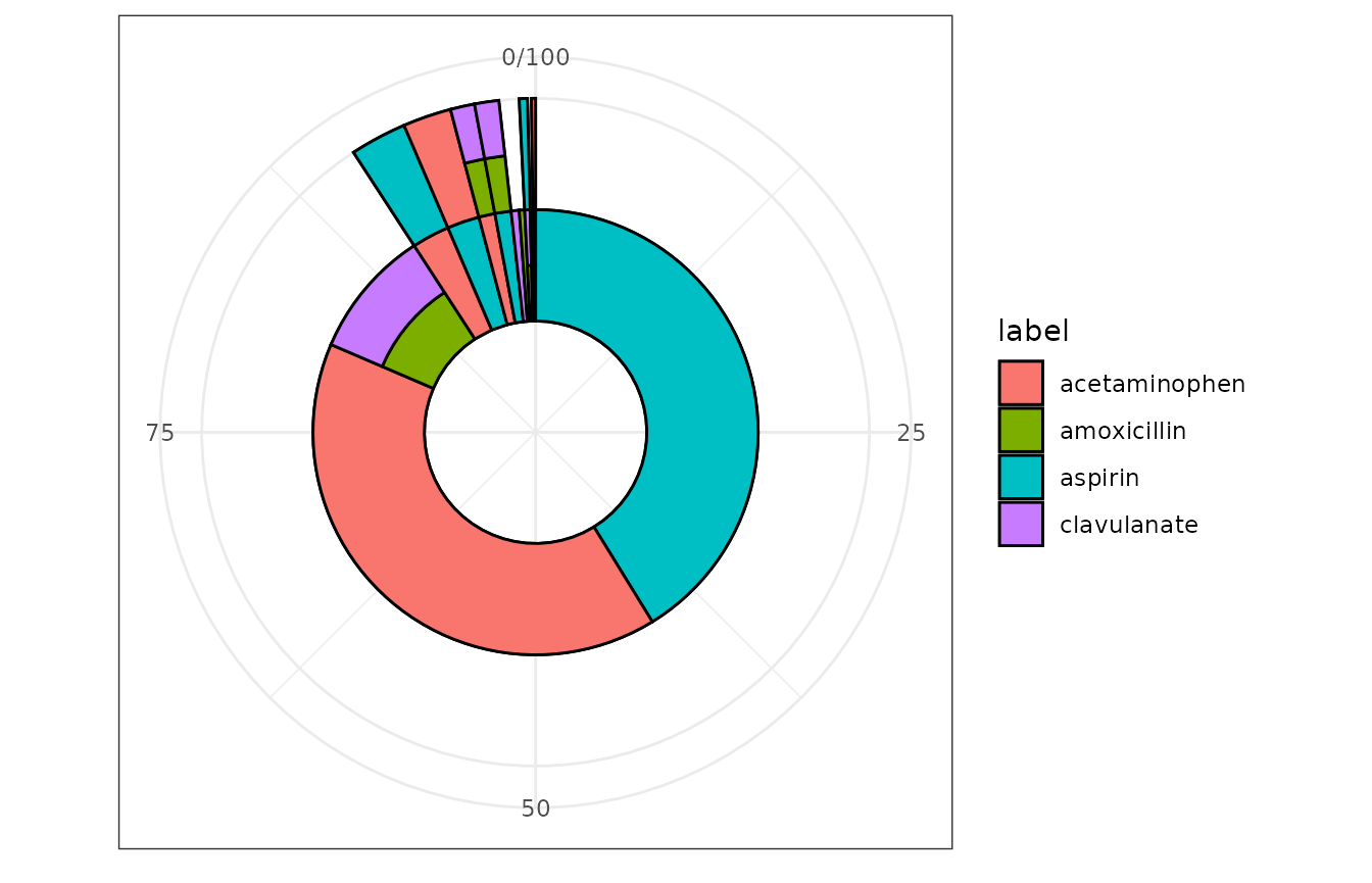

- Figure 4. Sankey diagram depicting treatment sequences after an index diagnosis.

TreatmentPatterns::createSankeyDiagram(treatmentPathways = treatmentPathways_data)