Using PatientProfiles for analysis • PatientProfiles

Set up

Let’s start by loading required packages and creating a cdm reference to the Eunomia dataset.

library(DBI)
library(duckdb)
library(CDMConnector)
library(omopgenerics)
library(CodelistGenerator)
library(dplyr)
library(PatientProfiles)
library(ggplot2)

con <- dbConnect(duckdb(), eunomia_dir())

cdm <- cdm_from_con(
  con = con, cdm_name = "eunomia", cdm_schema = "main", write_schema = "main"
)

Create bespoke cohorts

To start, we’ll define two drug cohorts. These cohorts will include drug exposures of celecoxib and diclofenac, respectively. To keep things simple each cohort entry will correspond to a drug exposure record (i.e. an individual can enter the cohort multiple times and we won’t concatenate any records). We’ll include these two cohorts in the same cohort table, with a cohort definition id of 1 for celecoxib and 2 for diclofenac.

For both cohorts we’ll also require that those included are aged between 40 and 50. The addAge function will facilitate incorporating this requirement.

celecoxibCodes <- getDescendants(cdm, conceptId = 1118084)
diclofenacCodes <- getDescendants(cdm, conceptId = 1124300)

# celecoxib
cdm$celecoxib <- cdm$drug_era %>%
  inner_join(
    celecoxibCodes %>%
      select(concept_id),
    by = c("drug_concept_id" = "concept_id"),
    copy = TRUE
  ) %>%
  addInObservation(indexDate = "drug_era_start_date") %>%
  filter(in_observation == 1) %>%
  addAge(indexDate = "drug_era_start_date") %>%
  filter(age >= 40 & age <= 50) %>%
  rename(
    "subject_id" = "person_id",
    "cohort_start_date" = "drug_era_start_date",
    "cohort_end_date" = "drug_era_end_date"
  ) %>%
  mutate(cohort_definition_id = 1L) %>%
  select(
    "cohort_definition_id", "subject_id",
    "cohort_start_date", "cohort_end_date"
  ) %>%
  compute()

# diclofenac
cdm$diclofenac <- cdm$drug_era %>%
  inner_join(
    diclofenacCodes %>%
      select(concept_id),
    by = c("drug_concept_id" = "concept_id"),
    copy = TRUE
  ) %>%
  addInObservation(indexDate = "drug_era_start_date") %>%
  filter(in_observation == 1) %>%
  addAge(indexDate = "drug_era_start_date") %>%
  filter(age >= 40 & age <= 50) %>%
  rename(
    "subject_id" = "person_id",
    "cohort_start_date" = "drug_era_start_date",
    "cohort_end_date" = "drug_era_end_date"
  ) %>%
  mutate(cohort_definition_id = 2L) %>%
  select(
    "cohort_definition_id", "subject_id",
    "cohort_start_date", "cohort_end_date"
  ) %>%
  compute()

cdm$exposure_cohort <- union_all(cdm$celecoxib, cdm$diclofenac) %>%
  compute(name = "exposure_cohort", temporary = FALSE) |>
  newCohortTable(cohortSetRef = tibble(
    cohort_definition_id = c(1, 2), cohort_name = c("celecoxib", "diclofenac")
  ))

As well as our two drug cohorts, we’ll define a cohort of people with a condition occurrence of gastrointestinal (GI) bleeding.

giBleedCodes <- getDescendants(cdm, conceptId = 192671)

# gi_bleed
cdm$gi_bleed <- cdm$condition_occurrence %>%
  inner_join(
    giBleedCodes %>%
      select(concept_id),
    by = c("condition_concept_id" = "concept_id"),
    copy = TRUE
  ) %>%
  rename(
    "subject_id" = "person_id",
    "cohort_start_date" = "condition_start_date"
  ) %>%
  mutate(cohort_end_date = cohort_start_date) %>%
  mutate(cohort_definition_id = 1L) %>%
  select(
    "cohort_definition_id", "subject_id",
    "cohort_start_date", "cohort_end_date"
  ) %>%
  compute(name = "gi_bleed", temporary = FALSE) |>
  newCohortTable(cohortSetRef = tibble(
    cohort_definition_id = 1, cohort_name = "gi_bleed"
  ))

Summarising cohort characteristics

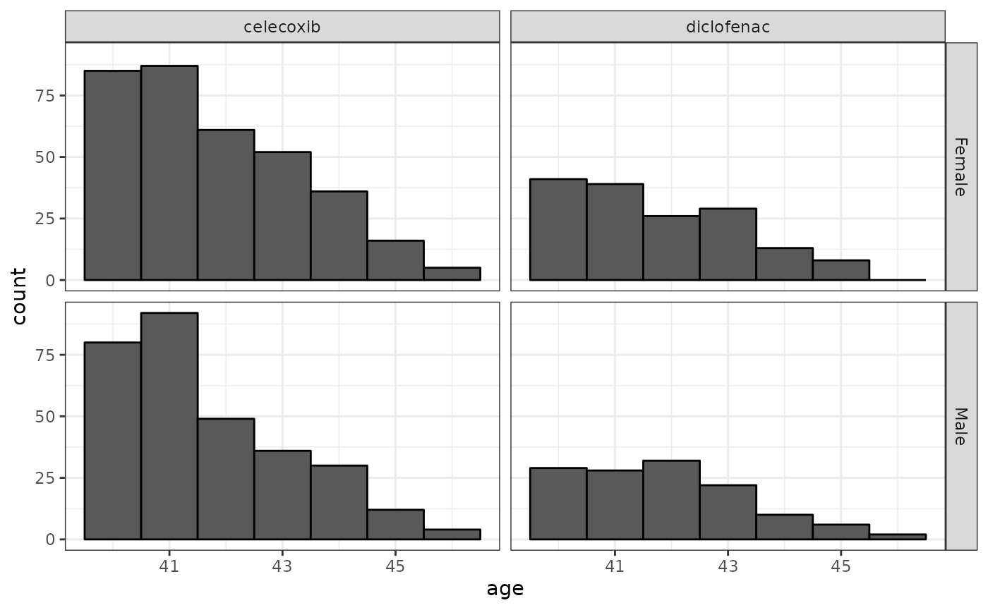
We can use the addDemographics to help describe the characteristics of our cohorts

cdm$exposure_cohort %>%
  addDemographics() %>%
  collect() %>%
  mutate(name = case_when(
    cohort_definition_id == 1 ~ "celecoxib",
    cohort_definition_id == 2 ~ "diclofenac",
    .default = as.character(cohort_definition_id)
  )) %>%
  collect() %>%
  ggplot() +
  facet_grid(sex ~ name) +
  geom_histogram(aes(age),
    binwidth = 1,
    colour = "black"
  ) +
  theme_bw()

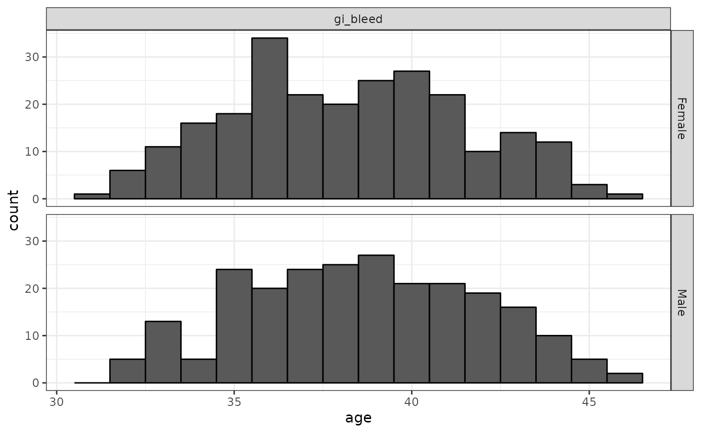
cdm$gi_bleed %>%
  addDemographics() %>%
  collect() %>%
  mutate(name = case_when(
    cohort_definition_id == 1 ~ "gi_bleed",
    .default = as.character(cohort_definition_id)
  )) %>%
  collect() %>%
  ggplot() +
  facet_grid(sex ~ name) +
  geom_histogram(aes(age),
    binwidth = 1,
    colour = "black"
  ) +
  theme_bw()

Cohort intersection

We can also see whether individuals had GI bleeding in some time period relative to their cohort start date using the flagCohortPresence function. In this case we’ll look at two time periods, before their cohort start date and after.

cdm$exposure_cohort <- cdm$exposure_cohort %>%
  addCohortIntersectFlag(
    targetCohortTable = "gi_bleed",
    indexDate = "cohort_start_date",
    window = c(-Inf, -1),
    nameStyle = "gi_bleed_history"
  ) %>%
  addCohortIntersectFlag(
    targetCohortTable = "gi_bleed",
    indexDate = "cohort_start_date",
    window = c(0, Inf),
    nameStyle = "gi_bleed_outcome"
  )

cdm$exposure_cohort %>%
  group_by(gi_bleed_history, gi_bleed_outcome) %>%
  count() %>%
  collect()
#> # A tibble: 2 × 3
#> # Groups:   gi_bleed_history, gi_bleed_outcome [2]
#>   gi_bleed_history gi_bleed_outcome     n
#>              <dbl>            <dbl> <dbl>
#> 1                0                0   754
#> 2                0                1   176

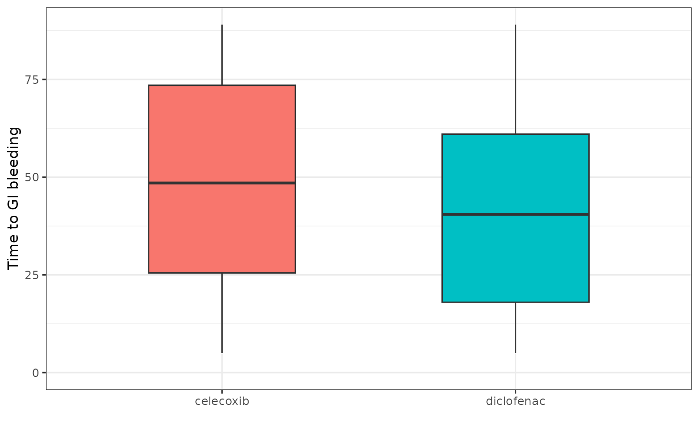
We can also see time to GI bleeding using the timeToCohort

cdm$exposure_cohort %>%
  addCohortIntersectDays(
    targetCohortTable = "gi_bleed",
    window = c(0, Inf),
    nameStyle = "time_to_event"
  ) %>%
  mutate(name = case_when(
    cohort_definition_id == 1 ~ "celecoxib",
    cohort_definition_id == 2 ~ "diclofenac",
    .default = as.character(cohort_definition_id)
  )) %>%
  group_by(name) %>%
  summarise(
    min_time_to_event = min(time_to_event, na.rm = TRUE),
    q25_time_to_event = quantile(time_to_event, 0.25, na.rm = TRUE),
    median_time_to_event = median(time_to_event, na.rm = TRUE),
    q75_time_to_event = quantile(time_to_event, 0.75, na.rm = TRUE),
    max_time_to_event = max(time_to_event, na.rm = TRUE)
  ) %>%
  collect() %>%
  ggplot(aes(
    x = name, group = name,
    fill = name
  )) +
  geom_boxplot(
    aes(
      lower = q25_time_to_event,
      upper = q75_time_to_event,
      middle = median_time_to_event,
      ymin = min_time_to_event,
      ymax = max_time_to_event
    ),
    stat = "identity", width = 0.5
  ) +
  theme_bw() +
  theme(legend.position = "none") +
  ylim(0, NA) +
  xlab("") +
  ylab("Time to GI bleeding")