Computing Treatment Pathways • TreatmentPatterns

In 1. Defining Cohorts we discussed how to define and generate cohorts for TreatmentPatterns. In this section we assume you are able to generate a cohort table using either CohortGenerator or CDMConnector.

Lets generate our Viral Sinusitis dummy cohorts provided in TreatmentPatterns using CDMConnector.

Generating Cohorts

First we need to read in our cohorts.

library(CDMConnector)

cohortSet <- readCohortSet(
  path = system.file(package = "TreatmentPatterns", "exampleCohorts")
)

cohortSet

## # A tibble: 8 × 5
##   cohort_definition_id cohort_name    cohort       json   cohort_name_snakecase
##                  <int> <chr>          <list>       <list> <chr>                
## 1                    1 acetaminophen  <named list> <chr>  acetaminophen        
## 2                    2 amoxicillin    <named list> <chr>  amoxicillin          
## 3                    3 aspirin        <named list> <chr>  aspirin              
## 4                    4 clavulanate    <named list> <chr>  clavulanate          
## 5                    5 death          <named list> <chr>  death                
## 6                    6 doxylamine     <named list> <chr>  doxylamine           
## 7                    7 penicillinv    <named list> <chr>  penicillinv          
## 8                    8 viralsinusitis <named list> <chr>  viralsinusitis

Then we can open a connection to our database, in this case Eunomia.

## 
## Attaching package: 'Eunomia'

## The following object is masked from 'package:CDMConnector':
## 
##     downloadEunomiaData

## 
## Download completed!

con <- DBI::dbConnect(
  drv = duckdb::duckdb(),
  dbdir = eunomia_dir()
)

## Warning: `eunomia_dir()` was deprecated in CDMConnector 1.7.0.
## ℹ Please use `eunomiaDir()` instead.
## This warning is displayed once every 8 hours.
## Call `lifecycle::last_lifecycle_warnings()` to see where this warning was
## generated.

## Creating CDM database /tmp/RtmpCN9Wxq/file26ef3c496c80/GiBleed_5.3.zip

cdm <- cdmFromCon(
  con = con,
  cdmSchema = "main",
  writeSchema = "main"
)

## Note: method with signature 'DBIConnection#Id' chosen for function 'dbExistsTable',
##  target signature 'duckdb_connection#Id'.
##  "duckdb_connection#ANY" would also be valid
## ! cdm name not specified and could not be inferred from the cdm source table

cdm

## 
## ── # OMOP CDM reference (duckdb) of An OMOP CDM database ───────────────────────
## • omop tables: person, observation_period, visit_occurrence, visit_detail,
## condition_occurrence, drug_exposure, procedure_occurrence, device_exposure,
## measurement, observation, death, note, note_nlp, specimen, fact_relationship,
## location, care_site, provider, payer_plan_period, cost, drug_era, dose_era,
## condition_era, metadata, cdm_source, concept, vocabulary, domain,
## concept_class, concept_relationship, relationship, concept_synonym,
## concept_ancestor, source_to_concept_map, drug_strength
## • cohort tables: -
## • achilles tables: -
## • other tables: -

Finally we can generate our cohort set as a cohort table into the database

cdm <- generateCohortSet(
  cdm = cdm,
  cohortSet = cohortSet,
  name = "cohort_table",
  overwrite = TRUE
)

## ℹ Generating 8 cohorts

## ℹ Generating cohort (1/8) - acetaminophen

## ✔ Generating cohort (1/8) - acetaminophen [359ms]

##

## ℹ Generating cohort (2/8) - amoxicillin

## ✔ Generating cohort (2/8) - amoxicillin [181ms]

##

## ℹ Generating cohort (3/8) - aspirin

## ✔ Generating cohort (3/8) - aspirin [166ms]

##

## ℹ Generating cohort (4/8) - clavulanate

## ✔ Generating cohort (4/8) - clavulanate [157ms]

##

## ℹ Generating cohort (5/8) - death

## ✔ Generating cohort (5/8) - death [120ms]

##

## ℹ Generating cohort (6/8) - doxylamine

## ✔ Generating cohort (6/8) - doxylamine [147ms]

##

## ℹ Generating cohort (7/8) - penicillinv

## ✔ Generating cohort (7/8) - penicillinv [154ms]

##

## ℹ Generating cohort (8/8) - viralsinusitis

## ✔ Generating cohort (8/8) - viralsinusitis [228ms]

##

cohortCount(cdm$cohort_table)

## # A tibble: 8 × 3
##   cohort_definition_id number_records number_subjects
##                  <int>          <int>           <int>
## 1                    1           2679            2679
## 2                    2           2130            2130
## 3                    3           1927            1927
## 4                    4           2021            2021
## 5                    5              0               0
## 6                    6           1393            1393
## 7                    7           1732            1732
## 8                    8           2159            2159

We can see that all our cohorts are generated in the cohort table. The cohort with cohort_definition_id 5 has a count of 0, this is the Death cohort. This is not detrimental, as exit cohorts are optional, but good to know that Death will not show up in our results.

Computing pathways

The computePathways function of TreatmentPatterns allows us to compute treatment pathways in our cohort table. In order to do this we need to pre-specify some parameters.

According to the documentation we need a data.frame that specifies what cohort is of which type.

Data frame containing the following columns and data types:

cohortId numeric(1) Cohort ID’s of the cohorts to be used in the cohort table.

cohortName character(1) Cohort names of the cohorts to be used in the cohort table.

type character(1) [“target”, “event’,”exit”] Cohort type, describing if the cohort is a target, event, or exit cohort

We are able to re-use our cohortSet for this. As it already contains the cohort ID’s and cohort names. We only have to remove the cohort and json columns, add a type column, and rename cohort_definition_id to cohortId and cohort_name to cohortName.

library(dplyr)

cohorts <- cohortSet %>%
  # Remove 'cohort' and 'json' columns
  select(-"cohort", -"json", -"cohort_name_snakecase") %>%
  mutate(type = c("event", "event", "event", "event", "exit", "event", "event", "target")) %>%
  rename(
    cohortId = "cohort_definition_id",
    cohortName = "cohort_name",
  )

cohorts

## # A tibble: 8 × 3
##   cohortId cohortName     type  
##      <int> <chr>          <chr> 
## 1        1 acetaminophen  event 
## 2        2 amoxicillin    event 
## 3        3 aspirin        event 
## 4        4 clavulanate    event 
## 5        5 death          exit  
## 6        6 doxylamine     event 
## 7        7 penicillinv    event 
## 8        8 viralsinusitis target

With our data.frame of cohort types, CDM reference, and the cohort table name in our database we can compute the treatment pathways, with all of the other settings as their defaults.

library(TreatmentPatterns)

defaultSettings <- computePathways(
  cohorts = cohorts,
  cohortTableName = "cohort_table",
  cdm = cdm
)

## -- Qualifying records for cohort definitions: 1, 2, 3, 4, 5, 6, 7, 8
##  Records: 14041
##  Subjects: 2693

## -- Removing records < minEraDuration (0)
##  Records: 11386
##  Subjects: 2159

## >> Starting on target: 8 (viralsinusitis)

## -- Removing events where index date < target index date + indexDateOffset (0)
##  Records: 8381
##  Subjects: 2159

## -- splitEventCohorts
##  Records: 8366
##  Subjects: 2144

## -- Collapsing eras, eraCollapse (30)
##  Records: 8366
##  Subjects: 2144

## -- Iteration 1: minPostCombinationDuration (30), combinatinoWindow (30)
##  Records: 558
##  Subjects: 512

## -- Iteration 2: minPostCombinationDuration (30), combinatinoWindow (30)
##  Records: 554
##  Subjects: 512

## -- After Combination
##  Records: 554
##  Subjects: 512

## -- filterTreatments (First)
##  Records: 553
##  Subjects: 512

## -- treatment construction done
##  Records: 553
##  Subjects: 512

defaultSettings

## # Andromeda object
## # Physical location:  /tmp/RtmpCN9Wxq/file26ef7a1f64fe.sqlite
## 
## Tables:
## $addRowsFRFS_1 (personId, indexYear, eventCohortId, eventStartDate, eventEndDate, type, age, sex, targetCohortId, durationEra, sortOrder, gapPrevious, selectedRows, switch, combinationFRFS, combinationLRFS, eventStartDateNext, eventEndDatePrevious, eventEndDateNext, eventCohortIdPrevious)
## $addRowsFRFS_2 (personId, indexYear, eventCohortId, targetCohortId, eventStartDate, age, sex, eventEndDate, durationEra, gapPrevious, sortOrder, selectedRows, switch, combinationFRFS, combinationLRFS, eventStartDateNext, eventEndDatePrevious, eventEndDateNext, eventCohortIdPrevious)
## $addRowsLRFS_1 (personId, indexYear, eventCohortId, eventStartDate, eventEndDate, type, age, sex, targetCohortId, durationEra, sortOrder, gapPrevious, selectedRows, switch, combinationFRFS, combinationLRFS, eventStartDateNext, eventEndDatePrevious, eventEndDateNext, eventCohortIdPrevious, checkDuration)
## $addRowsLRFS_2 (personId, indexYear, eventCohortId, targetCohortId, eventStartDate, age, sex, eventEndDate, durationEra, gapPrevious, sortOrder, selectedRows, switch, combinationFRFS, combinationLRFS, eventStartDateNext, eventEndDatePrevious, eventEndDateNext, eventCohortIdPrevious, checkDuration)
## $analyses (analysis_id, description)
## $arguments (analysis_id, arguments)
## $attrition (number_records, number_subjects, reason_id, reason, time_stamp)
## $cdm_source_info (cdm_source_name, cdm_source_abbreviation, cdm_holder, source_description, source_documentation_reference, cdm_etl_reference, source_release_date, cdm_release_date, cdm_version, vocabulary_version)
## $cohortTable (cohortId, personId, subject_id_origin, startDate, endDate, age, sex)
## $cohortTable_8 (cohortIdEvent, personId, subject_id_origin, startDateEvent, endDateEvent, ageEvent, sexEvent, typeEvent, cohortIdTarget, startDateTarget, endDateTarget, ageTarget, sexTarget, typeTarget, indexYear, indexDate)
## $cohorts (cohortId, cohortName, type)
## $currentCohorts (cohortId, personId, subject_id_origin, startDate, endDate, age, sex)
## $dbplyr_1WRZorR1u5 (number_records, number_subjects, reason_id, reason, time_stamp)
## $dbplyr_5pWJOAFS8a (number_records, number_subjects, reason_id, reason, time_stamp)
## $dbplyr_6RTXYj8SWn (number_records, number_subjects, reason_id, reason, time_stamp)
## $dbplyr_9H5PXKstDn (number_records, number_subjects, reason_id, reason, time_stamp)
## $dbplyr_BD55Q9nvAe (number_records, number_subjects, reason_id, reason, time_stamp)
## $dbplyr_KndACw8jLb (number_records, number_subjects, reason_id, reason, time_stamp)
## $dbplyr_c6hVi7vmXr (number_records, number_subjects, reason_id, reason, time_stamp)
## $dbplyr_g2ZRmBV2zb (number_records, number_subjects, reason_id, reason, time_stamp)
## $dbplyr_hYqzXdzCNp (number_records, number_subjects, reason_id, reason, time_stamp)
## $dbplyr_oLvteQFdqV (number_records, number_subjects, reason_id, reason, time_stamp)
## $eventCohorts (cohortId, personId, subject_id_origin, startDate, endDate, age, sex, type)
## $exitCohorts (cohortId, personId, subject_id_origin, startDate, endDate, age, sex, type)
## $exitHistory (personId, indexYear, eventCohortId, eventStartDate, eventEndDate, age, sex, targetCohortId, durationEra)
## $labels (eventCohortId, eventCohortName)
## $metadata (execution_start, package_version, r_version, platform, execution_end)
## $sqlite_stat1 (tbl, idx, stat)
## $sqlite_stat4 (tbl, idx, neq, nlt, ndlt, sample)
## $targetCohorts (cohortId, personId, subject_id_origin, startDate, endDate, age, sex, type, indexYear, indexDate)
## $treatmentHistory (eventCohortId, personId, indexYear, targetCohortId, eventStartDate, age, sex, eventEndDate, durationEra, sortOrder, eventSeq, eventCohortName)
## $treatmentHistoryFinal (eventCohortId, personId, indexYear, targetCohortId, eventStartDate, age, sex, eventEndDate, durationEra, sortOrder, eventSeq, eventCohortName)

The output of computePathways is an Andromeda environment, which allows us to investigate intermediate results and patient-level data. This data is not sharable.

# treatmentHistory table
head(defaultSettings$treatmentHistory)

## # Source:   SQL [?? x 12]
## # Database: sqlite 3.47.1 [/tmp/RtmpCN9Wxq/file26ef7a1f64fe.sqlite]
##   eventCohortId personId indexYear targetCohortId eventStartDate   age sex   
##   <chr>            <dbl>     <dbl>          <int>          <int> <dbl> <chr> 
## 1 1                   35      1961              8          -3073     2 MALE  
## 2 1                   10      1960              8          -3589     4 FEMALE
## 3 1                  625      1960              8           -510    13 FEMALE
## 4 1                  898      1969              8           4934    16 MALE  
## 5 1                  723      1957              8           1235    18 MALE  
## 6 1                  684      1979              8           4999    18 MALE  
## # ℹ 5 more variables: eventEndDate <int>, durationEra <int>, sortOrder <dbl>,
## #   eventSeq <int>, eventCohortName <chr>

# metadata table
defaultSettings$metadata

## # Source:   table<`metadata`> [?? x 5]
## # Database: sqlite 3.47.1 [/tmp/RtmpCN9Wxq/file26ef7a1f64fe.sqlite]
##   execution_start package_version r_version               platform execution_end
##             <dbl> <chr>           <chr>                   <chr>            <dbl>
## 1     1738853987. 3.0.0           R version 4.4.2 (2024-… x86_64-…   1738853994.

# First Recieved First Stopped
head(defaultSettings$addRowsFRFS_1)

## # Source:   SQL [?? x 20]
## # Database: sqlite 3.47.1 [/tmp/RtmpCN9Wxq/file26ef7a1f64fe.sqlite]
## # ℹ 20 variables: personId <lgl>, indexYear <dbl>, eventCohortId <lgl>,
## #   eventStartDate <int>, eventEndDate <lgl>, type <lgl>, age <dbl>, sex <chr>,
## #   targetCohortId <int>, durationEra <lgl>, sortOrder <lgl>,
## #   gapPrevious <lgl>, selectedRows <lgl>, switch <lgl>, combinationFRFS <lgl>,
## #   combinationLRFS <lgl>, eventStartDateNext <lgl>,
## #   eventEndDatePrevious <lgl>, eventEndDateNext <lgl>,
## #   eventCohortIdPrevious <lgl>

# Last Recieved Last Stopped
head(defaultSettings$addRowsLRFS_1)

## # Source:   SQL [?? x 21]
## # Database: sqlite 3.47.1 [/tmp/RtmpCN9Wxq/file26ef7a1f64fe.sqlite]
##   personId indexYear eventCohortId eventStartDate eventEndDate type    age sex  
##      <dbl>     <dbl> <chr>                  <int>        <int> <chr> <dbl> <chr>
## 1        5      1845 2                       9364         9364 event    31 MALE 
## 2        7      1227 2                       5965         5965 event    18 MALE 
## 3        8      -604 2                       7785         7785 event    28 MALE 
## 4       12      3657 2                      10855        10855 event    25 FEMA…
## 5       13      2202 2                       4512         4512 event     9 FEMA…
## 6       14      3877 1                       3891         3891 event     3 FEMA…
## # ℹ 13 more variables: targetCohortId <int>, durationEra <int>,
## #   sortOrder <dbl>, gapPrevious <int>, selectedRows <dbl>, switch <dbl>,
## #   combinationFRFS <dbl>, combinationLRFS <dbl>, eventStartDateNext <int>,
## #   eventEndDatePrevious <int>, eventEndDateNext <int>,
## #   eventCohortIdPrevious <chr>, checkDuration <dbl>

DatabaseConnector is also supported. The following parameters are required instead of cdm:

connectionDetails: ConnectionDetails object form DatabaseConnector.
cdmSchema: Schema where the CDM exists.
resultSchema: Schema to write the cohort table to.
tempEmulationSchema: Some database platforms like Oracle and Impala do not truly support temp tables. To emulate temp tables, provide a schema with write privileges where temp tables can be created.

The following code snippet works with Eunomia, a cohort table (cohort_table) exists in the database, and a cohorts data frame has been created.

computePathways(
  cohorts = cohorts,
  cohortTableName = cohortTableName,
  connectionDetails = Eunomia::getEunomiaConnectionDetails(),
  cdmSchema = "main",
  resultSchema = "main",
  tempEmulationSchema = NULL
)

Pathway settings

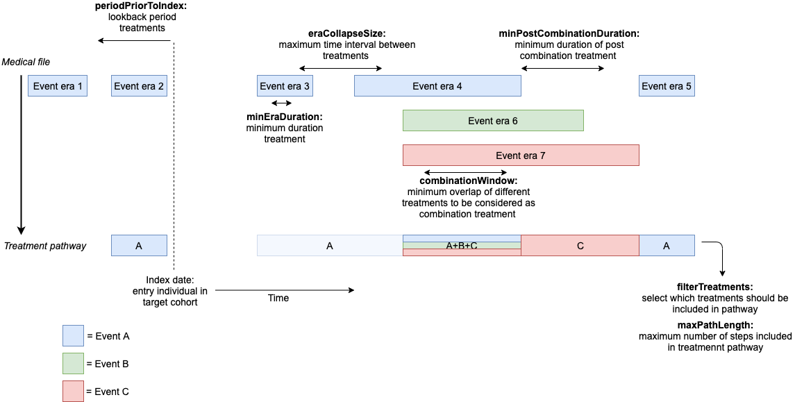
Even though the default settings work well for most use cases, it might not work for all situations. The settings below allow us to influence how the events of interest should be processed to form treatment pathways.

Parameter	Value	Description
indexDateOffset	0	Offset the index date of the `Target` cohort.
minEraDuration	0	Minimum time an event era should last to be included in analysis
eraCollapseSize	30	Window of time between which two eras of the same event cohort are collapsed into one era
combinationWindow	30	Window of time two event cohorts need to overlap to be considered a combination treatment
minPostCombinationDuration	30	Minimum time an event era before or after a generated combination treatment should last to be included in analysis
filterTreatments	First	Select first occurrence of (‘First’); changes between (‘Changes’); or all event cohorts (‘All’).
maxPathLength	5	Maximum number of steps included in treatment pathway

The following figure shows how each of these parameters affect the computation of the treatment pathway.

pathwaySettings You can add these settings to the computePathways function call. Lets see what happens when we set our minEraDuration to 60, but keep the rest of the settings mentioned as their default values.

minEra60 <- computePathways(
  cohorts = cohorts,
  cohortTableName = "cohort_table",
  cdm = cdm,
  # Pathway settings
  indexDateOffset = 0,
  minEraDuration = 60,
  eraCollapseSize = 30,
  combinationWindow = 30,
  minPostCombinationDuration = 30,
  filterTreatments = "First",
  maxPathLength = 5
)

## Warning in validateComputePathways(): The `minPostCombinationDuration` is set
## lower than the `minEraDuration`, this might result in unexpected behavior

## Warning in validateComputePathways(): The `combinationWindow` is set lower than
## the `minEraDuration`, this might result in unexpected behavior

## -- Qualifying records for cohort definitions: 1, 2, 3, 4, 5, 6, 7, 8
##  Records: 14041
##  Subjects: 2693

## -- Removing records < minEraDuration (60)
##  Records: 2523
##  Subjects: 2159

## >> Starting on target: 8 (viralsinusitis)

## -- Removing events where index date < target index date + indexDateOffset (0)
##  Records: 2216
##  Subjects: 2159

## -- splitEventCohorts
##  Records: 336
##  Subjects: 279

## -- Collapsing eras, eraCollapse (30)
##  Records: 336
##  Subjects: 279

## -- Iteration 1: minPostCombinationDuration (30), combinatinoWindow (30)
##  Records: 291
##  Subjects: 279

## -- After Combination
##  Records: 291
##  Subjects: 279

## -- filterTreatments (First)
##  Records: 291
##  Subjects: 279

## -- treatment construction done
##  Records: 291
##  Subjects: 279

Number of treatments with a minimum duration of greater or equal to 0 days.

defaultSettings$treatmentHistory %>%
  collect() %>%
  nrow()

## [1] 553

Number of treatments with a minimum duration of greater or equal to 60 days.

minEra60$treatmentHistory %>%
  collect() %>%
  nrow()

## [1] 291

Acute and Therapy splits

We can also split our defined event cohorts into acute and therapy cohorts.

Parameter	Description
splitEventCohorts	Specify event cohort ID’s (i.e. `c(1, 2, 3)` to split in acute (< splitTime days) and therapy (>= splitTime days). As an example treatment Drug A could be split into Drug A (therapy) and Drug A (acute). And we could set our splitTime to 30. Drug A (acute) would be the time before day 0-29 and Drug A (therapy) would be the day 30 or later.
splitTime	Specify number of days at which each of the split event cohorts should be split in acute and therapy (i.e. `c(20, 30, 10)`). The length of `splitTime` must equal the length of `splitEventCohorts`

Let’s say we want to assume that the first 60 days of our treatment is acute, and beyond that therapy.

splitAcuteTherapy <- computePathways(
  cohorts = cohorts,
  cohortTableName = "cohort_table",
  cdm = cdm,
  # Split settings
  splitEventCohorts = 1,
  splitTime = 60
)

## -- Qualifying records for cohort definitions: 1, 2, 3, 4, 5, 6, 7, 8
##  Records: 14041
##  Subjects: 2693

## -- Removing records < minEraDuration (0)
##  Records: 11386
##  Subjects: 2159

## >> Starting on target: 8 (viralsinusitis)

## -- Removing events where index date < target index date + indexDateOffset (0)
##  Records: 8381
##  Subjects: 2159

## -- splitEventCohorts
##  Records: 8366
##  Subjects: 2144

## -- Collapsing eras, eraCollapse (30)
##  Records: 8366
##  Subjects: 2144

## -- Iteration 1: minPostCombinationDuration (30), combinatinoWindow (30)
##  Records: 558
##  Subjects: 512

## -- Iteration 2: minPostCombinationDuration (30), combinatinoWindow (30)
##  Records: 554
##  Subjects: 512

## -- After Combination
##  Records: 554
##  Subjects: 512

## -- filterTreatments (First)
##  Records: 553
##  Subjects: 512

## -- treatment construction done
##  Records: 553
##  Subjects: 512

splitAcuteTherapy$treatmentHistory %>%
  pull(.data$eventCohortName) %>% unique()

## [1] "acetaminophen (acute)"             "acetaminophen (acute)+amoxicillin"
## [3] "acetaminophens (therapy)"          "amoxicillin"                      
## [5] "amoxicillin+clavulanate"           "aspirin"                          
## [7] "clavulanate"

We can see that our Acetaminophen cohorts are split into Acetaminophen (acute) and (therapy). Acute labels all the Acetaminophen cohorts lasting less than our defined splitTime, in this case 60 days. Therapy labels all the Acetaminophen cohorts lasting 60 days or more.

Include treatments in a time frame

We can dictate in what time frame we want to look. We can look from the start date of our target cohort and on wards, or we can look before the end date of our target cohort. By default TreatmentPatterns looks from the start date and onwards.

includeEndDate <- computePathways(
  cohorts = cohorts,
  cohortTableName = "cohort_table",
  cdm = cdm,
  # Split settings
  includeTreatments = "endDate"
)

## -- Qualifying records for cohort definitions: 1, 2, 3, 4, 5, 6, 7, 8
##  Records: 14041
##  Subjects: 2693

## -- Removing records < minEraDuration (0)
##  Records: 11386
##  Subjects: 2159

## >> Starting on target: 8 (viralsinusitis)

## -- Removing events where index date < target index date + indexDateOffset (0)
##  Records: 8381
##  Subjects: 2159

## -- splitEventCohorts
##  Records: 8366
##  Subjects: 2144

## -- Collapsing eras, eraCollapse (30)
##  Records: 8366
##  Subjects: 2144

## -- Iteration 1: minPostCombinationDuration (30), combinatinoWindow (30)
##  Records: 558
##  Subjects: 512

## -- Iteration 2: minPostCombinationDuration (30), combinatinoWindow (30)
##  Records: 554
##  Subjects: 512

## -- After Combination
##  Records: 554
##  Subjects: 512

## -- filterTreatments (First)
##  Records: 553
##  Subjects: 512

## -- treatment construction done
##  Records: 553
##  Subjects: 512

identical(
  includeEndDate$treatmentHistory %>% pull(personId),
  defaultSettings$treatmentHistory %>% pull(personId)
)

## [1] TRUE

In our example case for Viral Sinusitis it appears to not matter, as the personID’s are identical.

Exporting result objects

The export function allows us to export the generated result objects from computePathways. There are several arguments that we can change to alter the behavior, depending on what we are allowed to share.

minCellCount and censorType

Let’s say we are only able to share results of groups of subjects that have at least 5 subjects in them.

results <- export(
  andromeda = defaultSettings,
  minCellCount = 5
)

We can also choose between different methods how to handle pathways that fall below are specified minCellCount. These types are 1) "cellCount", 2) "remove", and 3) "mean".

We could say we want to censor all pathways that fall below the minCellCount to be censored to the minCellCount.

resultsA <- export(
  andromeda = minEra60,
  minCellCount = 5,
  censorType = "minCellCount"
)

Or we could completely remove them

resultsB <- export(
  andromeda = minEra60,
  minCellCount = 5,
  censorType = "remove"
)

Or finally we can censor them as the mean of all the groups that fall below the minCellCount.

resultsC <- export(
  andromeda = minEra60,
  minCellCount = 5,
  censorType = "mean"
)

ageWindow

We can also specify an age window.

resultsD <- export(
  andromeda = splitAcuteTherapy,
  minCellCount = 5,
  censorType = "mean",
  ageWindow = 3
)

Or a collection of ages.

resultsE <- export(
  andromeda = splitAcuteTherapy,
  minCellCount = 5,
  censorType = "mean",
  ageWindow = c(0, 18, 25, 30, 40, 50, 60, 150)
)

archiveName

Finally we can also specify an archiveName which is the name of a zip-file to zip all our output csv-files to.

resultsF <- export(
  andromeda = includeEndDate,
  minCellCount = 5,
  censorType = "mean",
  ageWindow = 3,
  archiveName = "output.zip"
)

All-in-one

Instead of using computePathways and export, instead we could use executeTreatmentPatterns. Which is an all-in-one function that trades full control for convenience.

resultsG <- executeTreatmentPatterns(
  cohorts = cohorts,
  cohortTableName = "cohort_table",
  cdm = cdm,
  minEraDuration = 0,
  eraCollapseSize = 30,
  combinationWindow = 30,
  minCellCount = 5
)

## -- Qualifying records for cohort definitions: 1, 2, 3, 4, 5, 6, 7, 8
##  Records: 14041
##  Subjects: 2693

## -- Removing records < minEraDuration (0)
##  Records: 11386
##  Subjects: 2159

## >> Starting on target: 8 (viralsinusitis)

## -- Removing events where index date < target index date + indexDateOffset (0)
##  Records: 8381
##  Subjects: 2159

## -- splitEventCohorts
##  Records: 8366
##  Subjects: 2144

## -- Collapsing eras, eraCollapse (30)
##  Records: 8366
##  Subjects: 2144

## -- Iteration 1: minPostCombinationDuration (30), combinatinoWindow (30)
##  Records: 558
##  Subjects: 512

## -- Iteration 2: minPostCombinationDuration (30), combinatinoWindow (30)
##  Records: 554
##  Subjects: 512

## -- After Combination
##  Records: 554
##  Subjects: 512

## -- filterTreatments (First)
##  Records: 553
##  Subjects: 512

## -- treatment construction done
##  Records: 553
##  Subjects: 512

## Censoring 1540 pathways with a frequency <5 to mean.

When using DatabaseConnector we can substitute the cdm object with connectionDetails, cdmSchema, resultSchema, and tempEmulationSchema.

executeTreatmentPatterns(
  cohorts = cohorts,
  cohortTableName = "cohort_table",
  connectionDetails = Eunomia::getEunomiaConnectionDetails(),
  cdmSchema = "main",
  resultSchema = "main",
  tempEmulationSchema = NULL,
  minEraDuration = 0,
  eraCollapseSize = 30,
  combinationWindow = 30,
  minCellCount = 5
)

Evaluating output

Now that we have exported our output, in various ways, we can evaluate the output. As you may have noticed the export function exports 6 csv-files: 1) treatmentPathways.csv, 2) countsAge.csv, 3) countsSex.csv, 4) countsYear.csv, 5) summaryStatsTherapyDuraion.csv, and 6) metadata.csv

treatmentPathways

The treatmentPathways file contains all the pathways found, with a frequency, pairwise stratified by age group, sex and index year.

results$treatment_pathways

## # A tibble: 12 × 8
##    pathway              freq age   sex   index_year analysis_id target_cohort_id
##    <chr>               <int> <chr> <chr> <chr>            <dbl>            <int>
##  1 aspirin               211 all   all   all                  1                8
##  2 acetaminophen         206 all   all   all                  1                8
##  3 amoxicillin+clavul…    48 all   all   all                  1                8
##  4 acetaminophen-aspi…    14 all   all   all                  1                8
##  5 aspirin-acetaminop…    12 all   all   all                  1                8
##  6 acetaminophen-amox…     6 all   all   all                  1                8
##  7 aspirin-amoxicilli…     6 all   all   all                  1                8
##  8 clavulanate             3 all   all   all                  1                8
##  9 amoxicillin             2 all   all   all                  1                8
## 10 amoxicillin+clavul…     2 all   all   all                  1                8
## 11 acetaminophen+amox…     1 all   all   all                  1                8
## 12 amoxicillin+clavul…     1 all   all   all                  1                8
## # ℹ 1 more variable: target_cohort_name <chr>

We can see the pathways contain the treatment names we provided in our event cohorts. Besides that we also see the paths are annoted with a + or -. The + indicates two treatments are a combination therapy, i.e. Acetaminophen+Amoxicillin is a combination of Acetaminophen and Amoxicillin. The - indicates a switch between treatments, i.e. Aspirin-Acetaminophen is a switch from Aspirin to Acetaminophen. Note that these combinations and switches can occur in the same pathway, i.e. Amoxicillin+Clavulanate-Aspirin. The first treatment is a combination of Amoxicillin and Clavulanate that switches to Aspirin.

countsAge, countsSex, and countsYear

The countsAge, countsSex, and countsYear contain counts per age, sex, and index year.

head(results$counts_age)

## # A tibble: 6 × 5
##     age n     analysis_id target_cohort_id target_cohort_name
##   <dbl> <chr>       <dbl>            <int> <chr>             
## 1     1 18              1                8 viralsinusitis    
## 2     2 55              1                8 viralsinusitis    
## 3     3 45              1                8 viralsinusitis    
## 4     4 37              1                8 viralsinusitis    
## 5     5 33              1                8 viralsinusitis    
## 6     6 32              1                8 viralsinusitis

head(results$counts_sex)

## # A tibble: 2 × 5
##   sex    n     analysis_id target_cohort_id target_cohort_name
##   <chr>  <chr>       <dbl>            <int> <chr>             
## 1 FEMALE 254             1                8 viralsinusitis    
## 2 MALE   258             1                8 viralsinusitis

head(results$counts_year)

## # A tibble: 6 × 5
##   index_year n     analysis_id target_cohort_id target_cohort_name
##        <dbl> <chr>       <dbl>            <int> <chr>             
## 1       1950 11              1                8 viralsinusitis    
## 2       1951 11              1                8 viralsinusitis    
## 3       1952 10              1                8 viralsinusitis    
## 4       1953 12              1                8 viralsinusitis    
## 5       1954 12              1                8 viralsinusitis    
## 6       1955 14              1                8 viralsinusitis

summaryStatsTherapyDuration

The summaryEventDuration file contains summary statistics from different events, across all found “lines”. A “line” is equal to the level in the Sunburst or Sankey diagrams. The summary statistics allow for plotting of boxplots with the plotEventDuration() function.

results$plotEventDuration()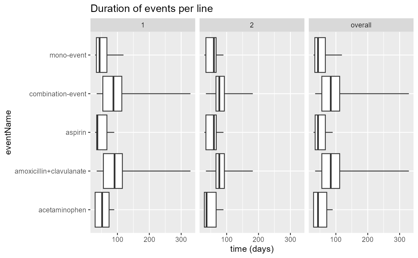

Or we can use the function

plotEventDuration(results$summary_event_duration)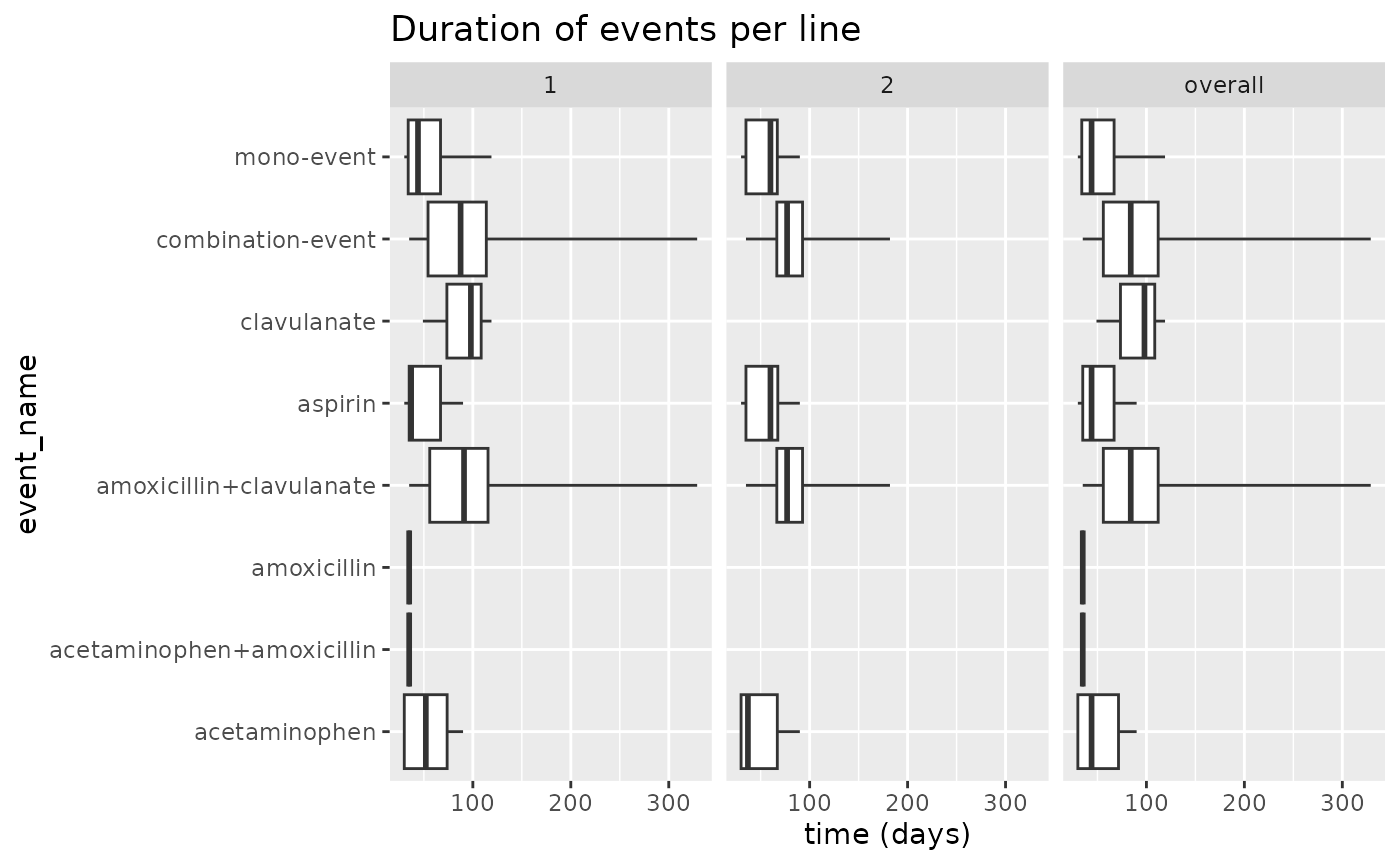

metadata

The metadata file is a file that contains information about the circumstances the analysis was performed in, and information about R, and the CDM.

results$metadata

## # A tibble: 1 × 6
##   execution_start package_version r_version   platform execution_end analysis_id
##             <dbl> <chr>           <chr>       <chr>            <dbl>       <dbl>
## 1     1738853987. 3.0.0           R version … x86_64-…   1738853994.           1

Sunburst Plot & Sankey Diagram

From the filtered treatmentPathways file we are able to create a sunburst plot.

results$plotSunburst()

Or a Sankey Diagram.

results$plotSankey()

Both plots are interactive in an HTML-environment, and are easy to include in shiny applications.